Representations of Dynamic Systems -- Problems of SEM / Regression / Discrete Time

Last updated on Nov 18, 2022 6 min read

Representing Dynamic Systems

Building on from the dynamic systems intro in a previous post, to build formal models of dynamic systems, we need some way to represent them mathematically. A common approach used in the social sciences is that of a ‘difference equation’, or ‘structural equation model’ (SEM), both of which are forms of a ‘discrete time’ representation. While such an approach is computationally appealing and familiar to most social scientists, it often does not represent the causal system that people think it does, and is problematic for scenarios where certain paths are fixed to zero, as with hypothesis testing or some forms of data driven structure determination.

Discrete time

In a discrete time model, changes are assumed to occur in discrete packets at certain points of time – usually at a specific time step, or interval. In most cases this time interval is based, for convenience, on the interval found in the observed data, for instance in the case of many large scale panel studies this might be 1 year. A 3 variable longitudinal SEM might look like this:

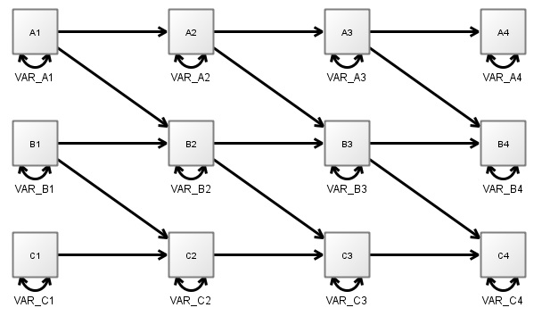
In this case, the model represents the state of the world where A (top variable) causes B (middle), which in turn causes C. Assuming yearly data, this implies that it takes 2 years for a change in A to begin to have any impact on C.

Problems with discrete time

If we take the exact same representation, but happen to have gathered data every week, then we actually have very different causal implications – our model would then imply that A begins to influence C after 2 weeks.
This is a problem! In most cases this is not what we want from a model. For most constructs of interest, we generally assume that the constructs are always ‘there’, and continually exerting influence on other constructs in the system. If somebody changes their daily level of exercise, we know that yes, it will take some time to show meaningful change in fitness, but that the processes connecting a change in exercise habits to fitness begin to play out straight away. (Even in cases where it may not be straight away, there is rarely reason to think they play out discretely at the exact rate of data gathering!)

Time as an infinite stream of latent variables

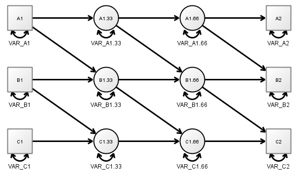
We could approximate such a scenario using a discrete time representation by inserting a lot of missing values in our data, for example, a missing value every minute. Then, instead of estimating the regression weight between each year, we would estimate it between each minute. While still not technically correct, at this point it’s very likely a close enough approximation. The following diagram depicts a limited form of this, ‘zooming in’ on the first 2 measureent occasions and showing 2 ‘missing value’ latent variables inserted between them – really, one needs to imagine an infinite succession of such latent variables between each observation however.

Once such missing values are included, the resulting pattern of regressions and covariances between the variables we’ve actually observed is much more connected than our hypothetical causal model! The following diagram represents the pattern we would expect in the case that A is causing B and B is causing C continuously. Note that both regressions and covariances become more connected / less sparse.

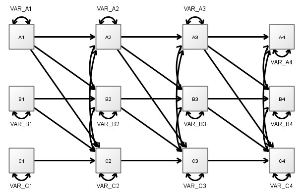
So, the implications of even a sparse model, once these play out repeatedly over time, result in a much more connected SEM / discrete time representation than our actual hypothesised model. This can be understood as follows: B is the only ‘direct’ cause of C, so one might think that knowing B at the earlier time point would contain all possible information about C at the next point. However, B is changing during the time between our first and second observations, and since A causes B, A contains information about the change in B. Thus, including knowledge of A (i.e. a non zero regression path) leads to improved estimates of C at the next point in time.
The mathematics of ‘including the missing values’ are well known for a long time, and the regression weights for a specific causal system can be easily computed by taking the causal / temporal / direct effect matrix, multiplying it by the time interval, and then taking the matrix exponential of the result. For the 3 variable system described above, the result looks like this, for the effect of a change in variable A on all three variables:

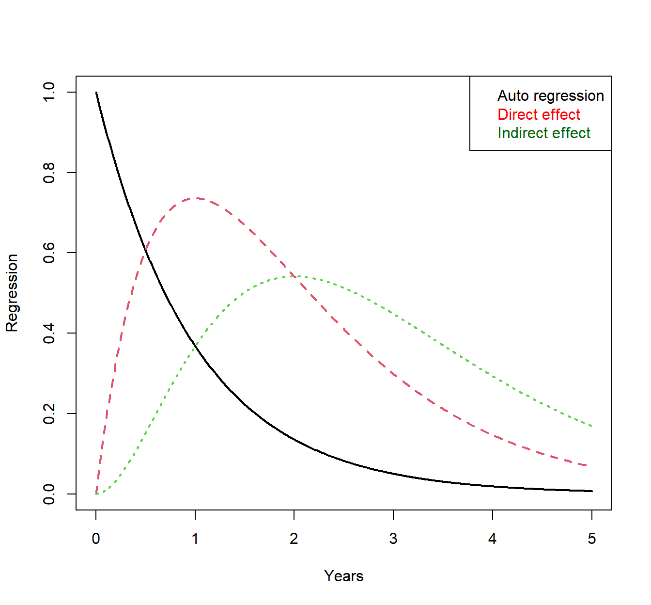
We see that once there is some change in variable A at time zero, because it is a typical mean reverting process (i.e. tends to head back towards some centre after some change), the predictiveness of time point zero on later time points begins to decline straight away – shown by the black auto regression plot. In contrast, a change in A at time zero is most noticeable in B after around a year, even though changes are indeed occurring straight away. This begins to make sense when you consider that because process A does not revert to the centre immediately, the initial change at time zero continues to exert influence. Peak change in variable C is later than for variable B for the same reason – after the peak change of variable B, variable B is still well above baseline and so continues to exert influence. Note that even though A does not directly influence C, C still changes immediately, if somewhat slower than B.

Implications

The core point of all this is that for a model with few direct connections between continuously interacting processes, there are usually far more indirect connections that result at a specific time interval. This means that while the discrete time / SEM approach works quite fine for contexts where all the connections are freely estimated and the goal is simply prediction, it is very difficult to specify coherent hypothesis regarding causal effects – which is generally the goal of SEM style approaches – because the regressions and covariances do not represent causal / direct effects! This is the case whenever variables are assumed to be continuously interacting, and does not depend on how slow or fast the interaction is.
A similar problem occurs when using penalisation approaches (e.g. lasso regularization) or Bayesian priors on the regression coefficients to find the ‘true structure’ of the system. Even to the extent that finding a sensible approximation to the true structure is possible with data driven approaches, shrinking the indirect (imagining many unobserved mediating variables at intermediate time points) paths to zero, is unlikely to get us there – one would instead need some way of penalising the causal effects directly, instead of penalasing the implications of such causal effects after some length of time.
Differential equations / continuous time approaches (e.g. ctsem), offer a neat way out of this conundrum – allowing us to specify the underlying pattern of direct / causal relationships, then solve the resulting equation for whatever pattern of observation time intervals we have in our data. Essentially, allowing for the sorts of causal specification and hypothesis testing (as difficult and problematic as this may be!) that people seem to think is possible using SEM / regression style approaches, but generally isn’t! More on differential equations next post…