Binary data in state space models
Generate some data
Here we specify a bivariate latent process where the 1st process affects the 2nd, and there are stable individual differences in the processes.
library(ctsem)
gm <- ctModel(LAMBDA=diag(2), #diagonal factor loading, 2 latents 2 observables
  Tpoints = 50,
  DRIFT=matrix(c(-1,.5,0,-1),2,2), #temporal dynamics
  TRAITVAR = diag(.5,2), #stable latent intercept variance (cholesky factor)
  DIFFUSION=diag(2)) #within person covariance

ctModelLatex(gm) #to view latex system equations

#when generating data, free pars are set to 0
d <- data.frame(ctGenerate(ctmodelobj = gm,n.subjects = 100,
  burnin = 20,dtmean = .1))
We didn’t specify any measurement error in the above code, because we’re going to mix the regular Gaussian approach with binary data measurements:
d$Y2binary <-rbinom(n = nrow(d),size = 1, #create binary data based on the latent
  prob = ctsem::inv_logit(d$Y2))
d$Y1 <- d$Y1 + rnorm(nrow(d),0,.2) #gaussian measurement error
Now we setup our model for estimation – we no longer hard code the values of the simulation! We also fix the MANIFESTMEANS (measurement intercept) and free the CINT (continuous / latent process intercept) because that will be more appropriate if there are stable differences in the latent process. In Gaussian cases this choice of how to identify the model very often makes no difference, but it is more crucial with non-linearity. Note that there are many system matrices left unspecified, which will be freely estimated by default, and note also that correlated individual differences are enabled by default for all intercept terms (in this case, inital latent process intercepts, and continuous intercepts). The final step is to specify the measurement model by altering the model object directly – once the binary feature gets more development time I will probably create a nicer approach for this. 0 for the first manifest specifies that it is Gaussian, while the 1 specifies that our second variable (listed in manifestNames) is binary.
m <- ctModel(LAMBDA=diag(2),type='stanct',
  manifestNames = c('Y1','Y2binary'),
  MANIFESTMEANS = 0,
  CINT=c('cint1','cint2'))
##      [,1]
## [1,]  "0"
## [2,]  "0"
##      [,1]
## [1,] "cint1"
## [2,] "cint2"

m$manifesttype=c(0,1)
Then we fit and summarise the model – note that at time of writing the latex output doesn’t know about the binary measurement model for the 2nd observable, and incorrectly shows the errors as Gaussian.
f <- ctStanFit(datalong = d,ctstanmodel = m,cores=6)
s=summary(f)
print(s$popmeans)
##                    mean     sd    2.5%     50%   97.5%
## T0m_eta1         0.1138 0.0907 -0.0650  0.1168  0.2798
## T0m_eta2        -0.1224 0.1155 -0.3534 -0.1259  0.1065
## drift_eta1      -0.9252 0.1277 -1.1902 -0.9146 -0.7104
## drift_eta1_eta2  0.1157 0.1728 -0.2206  0.1177  0.4593
## drift_eta2_eta1  1.0519 0.2989  0.4570  1.0510  1.6362
## drift_eta2      -1.0935 0.3588 -1.9238 -1.0557 -0.5062
## diff_eta1        0.9664 0.0289  0.9075  0.9655  1.0237
## diff_eta2_eta1  -0.0114 0.0762 -0.1605 -0.0081  0.1318
## diff_eta2        0.8806 0.1876  0.5844  0.8568  1.2874
## mvarY1           0.2016 0.0070  0.1878  0.2017  0.2157
## cint1            0.0238 0.0621 -0.0940  0.0252  0.1442
## cint2           -0.0990 0.0883 -0.2758 -0.0991  0.0782
ctModelLatex(f)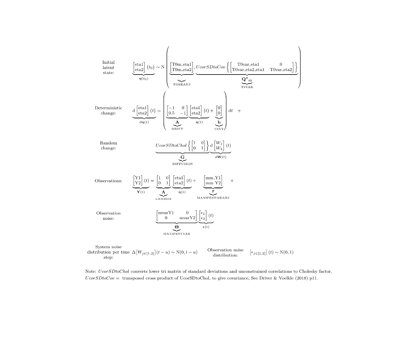
Then add a few plots showing temporal regression coefficients conditional on time interval, measurement expectations conditional on estimated parameters and past data, and finally latent states conditional on estimated parameters and both past and future data.
ctStanDiscretePars(f,plot=T)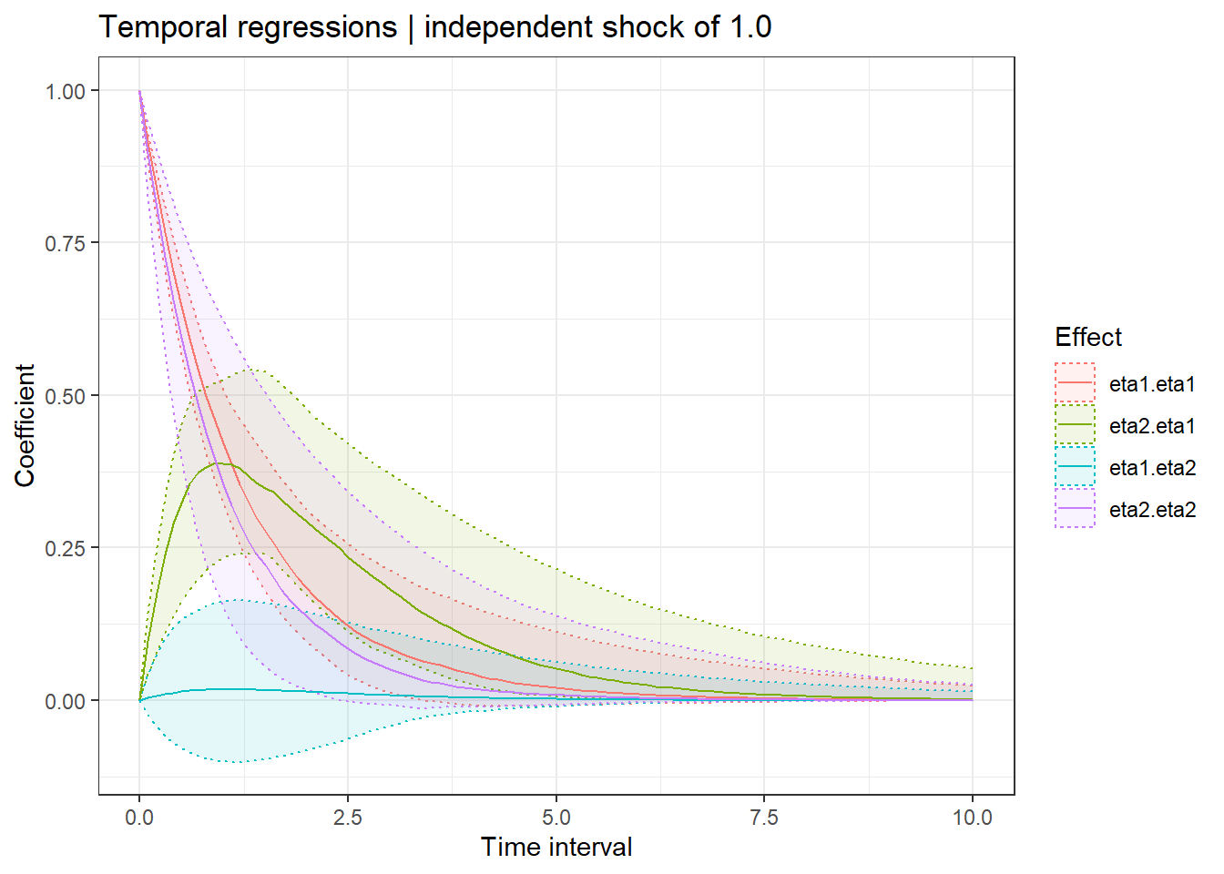
ctKalman(f,subjects = c(2,5),plot=T)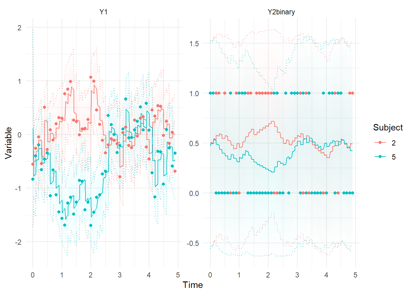
ctKalman(f,subjects = c(2,5),plot=T,kalmanvec=c('etasmooth'))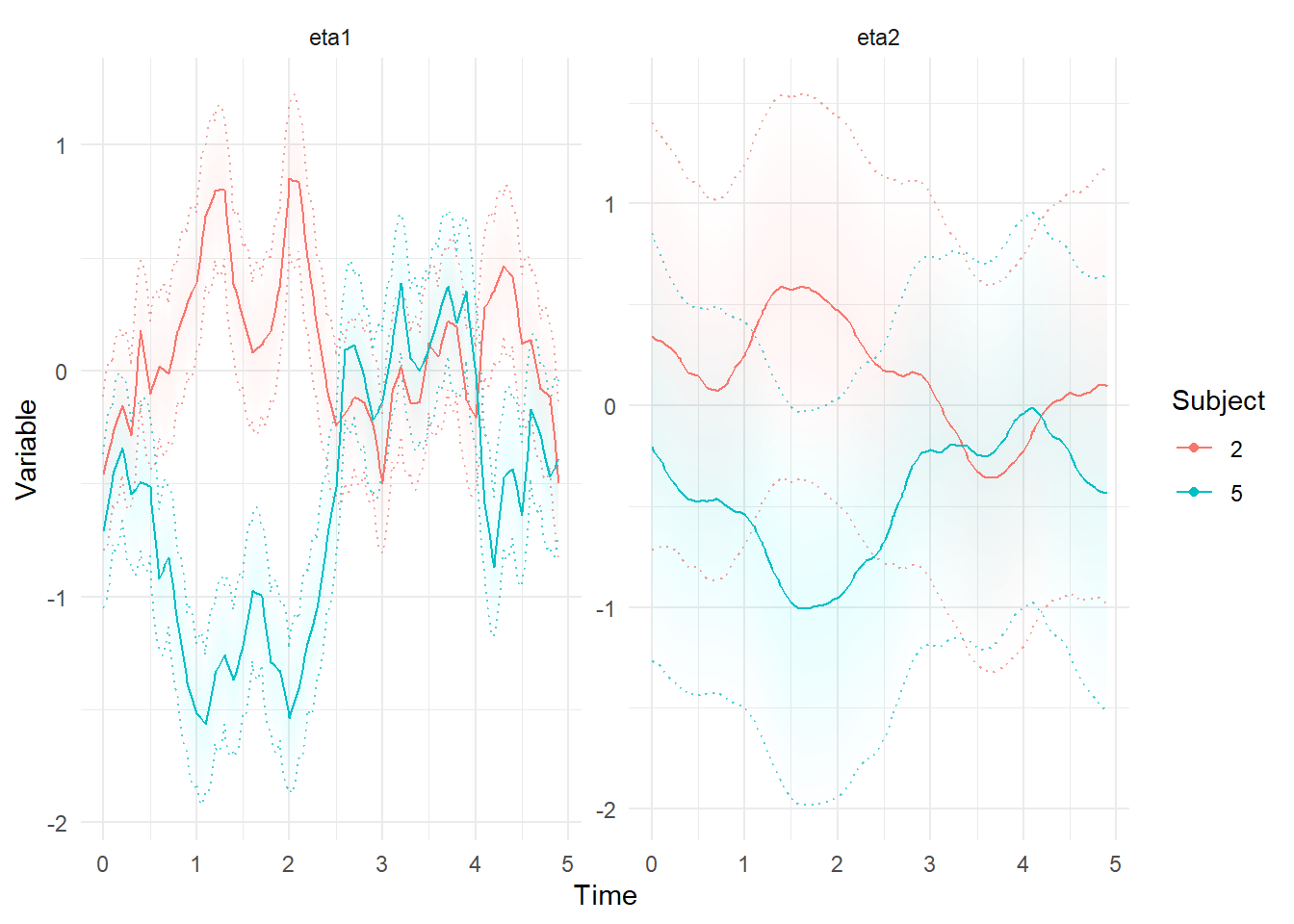
Charles Driver
Research Scientist
I’m a quantitative psychologist interested in the dynamic systems perspective of human systems.