Latent growth curves are a nice, relatively straightforward model for estimating overall patterns of change from multiple, noisy, indicator variables. While the classic formulations of this model can be easily fit in most SEM packages, it provides a nice basis for understanding the differential equation formulation of systems, and also a good starting point for more complex model development not possible in the SEM framework – as a peek into these possibilities I’ll also show a growth curve model where the measurement error depends on the latent variable, as would be typical of floor or ceiling effects.

To show this I’ll use ctsem. ctsem is R software for statistical modelling using hierarchical state space models, of discrete or continuous time formulations, with possible nonlinearities (ie state / time dependence) in the parameters. For a general quick start see https://cdriver.netlify.com/post/ctsem-quick-start/ , and for more details see the current manual at https://github.com/cdriveraus/ctsem/raw/master/vignettes/hierarchicalmanual.pdf

Data

Lets load ctsem (if you haven’t installed it see the quick start post!), and generate some data from a simple linear latent growth model.

set.seed(3)
library(ctsem)

nsubjects <- 30
nobs <- 8 #number of obs
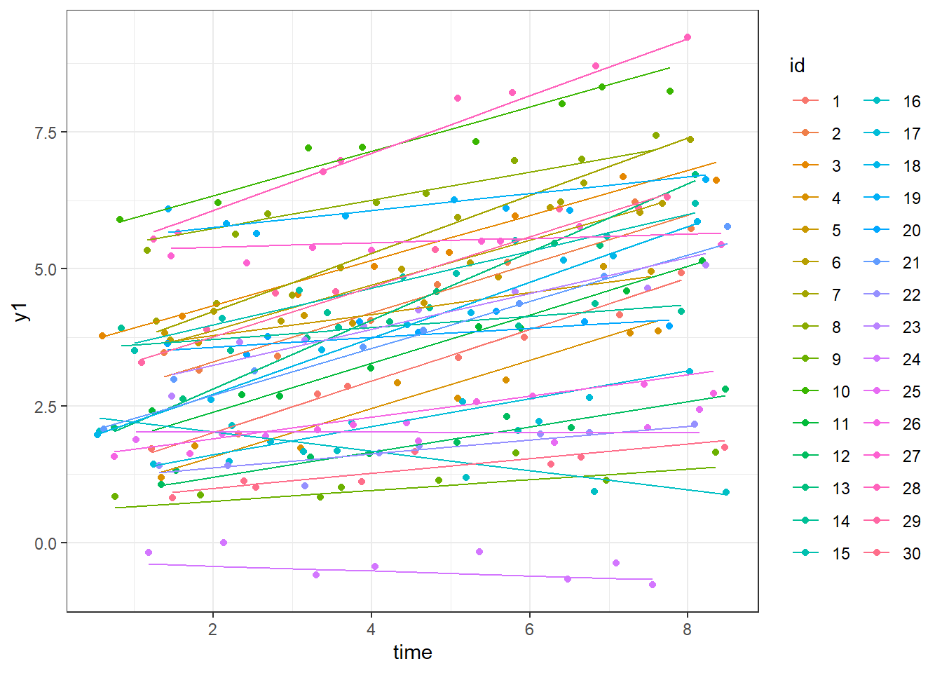
intercept <- rnorm(nsubjects, 3,2) #random intercepts
slope <- rnorm(nsubjects, .3, .2) - intercept * .01 #random slopes with intercept correlation
dat <- data.frame(matrix(NA,nrow=nsubjects*nobs,ncol=3)) #empty dataframe
colnames(dat) <- c('id','time','eta1')

r<-0
for(subi in 1:nsubjects){
  for(obsi in 1:nobs){
    r <- r+1 #current row
    dat$time[r] <- obsi + runif(1,-.5,.5) #observation timing variation
    dat$id[r] <- subi
    dat$eta1[r] <- intercept[subi] + dat$time[r] * slope[subi] 
  }
}
dat$y1 <- dat$eta1 + rnorm(nrow(dat),0,.2) #observed variable with measurement error
dat$id <- factor(dat$id)

head(dat)
##   id     time     eta1       y1
## 1  1 1.216853 1.647280 1.711899
## 2  1 2.322188 2.166084 1.988314
## 3  1 3.320742 2.634769 2.713504
## 4  1 3.699945 2.812753 2.860061
## 5  1 5.101135 3.470421 3.384321
## 6  1 5.929836 3.859382 3.749796

library(ggplot2)
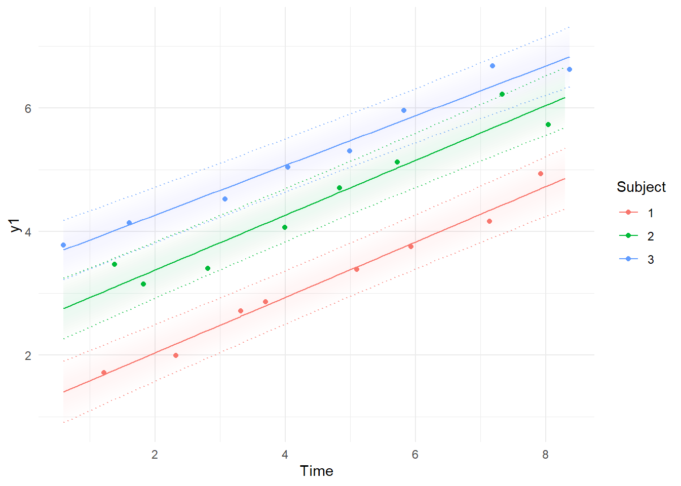
ggplot(dat,aes(y=y1,x=time,colour=id))+geom_point()+
  theme_bw()+geom_line(aes(y=eta1))

Model

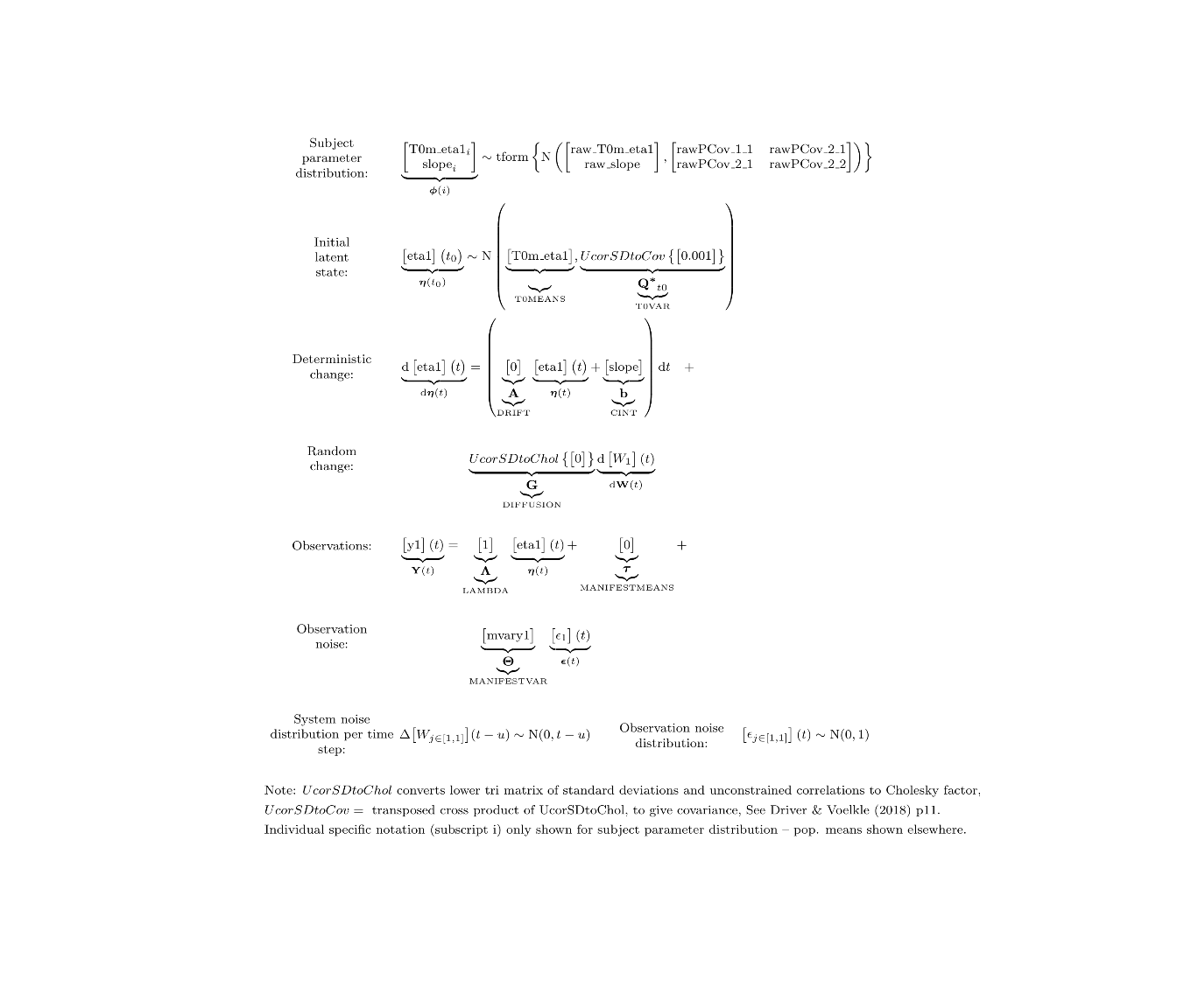
The default model in ctsem is rather more flexible than linear growth, so we need to impose some restrictions on the dynamic system model, such that the change in the latent variable at any particular point does not depend on the current value of the latent variable, but only on the slope (or continuous time intercept) parameter. This continuous intercept parameter is fixed to zero by default, and instead measurement intercepts are estimated – in this case we need to switch this. Since growth curve models also assume that changes in the latent variable are deterministic, we also need to restrict the system noise (diffusion) parameters to zero. In terms of individual differences, when multiple subjects are specified, the default is to have random (subject specific) initial states and intercepts (with correlation between the two), which is just fine for our current model. Since we have variation in the observation timing (both within and between subjects in this case) we need to use the continuous time, differential equation format. For growth curve models, the discrete time forms are exactly equivalent to continuous time when the time between observations is 1, of whatever time unit is being used.

model <- ctModel(type='stanct', # use 'standt' for a discrete time setup
  DRIFT=0,
  DIFFUSION=0,
  CINT='slope',
  MANIFESTMEANS=0,
  manifestNames='y1',latentNames='eta1',
  LAMBDA=1) #Factor loading fixed to 1

ctModelLatex(model) #requires latex install -- will prompt with instructions in any case

Fit

Fit using optimization and maximum likelihood (defaults as of v2.2.1):

fit<- ctStanFit(dat, model, cores=2) 

Summarise / Visualise

Then we can use various summary and plotting functions:

ctModelLatex(fit) #requires latex install -- will prompt with instructions in any case

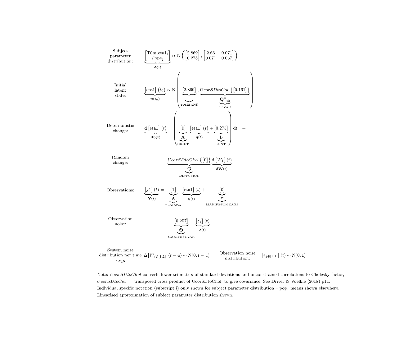
summary(fit)

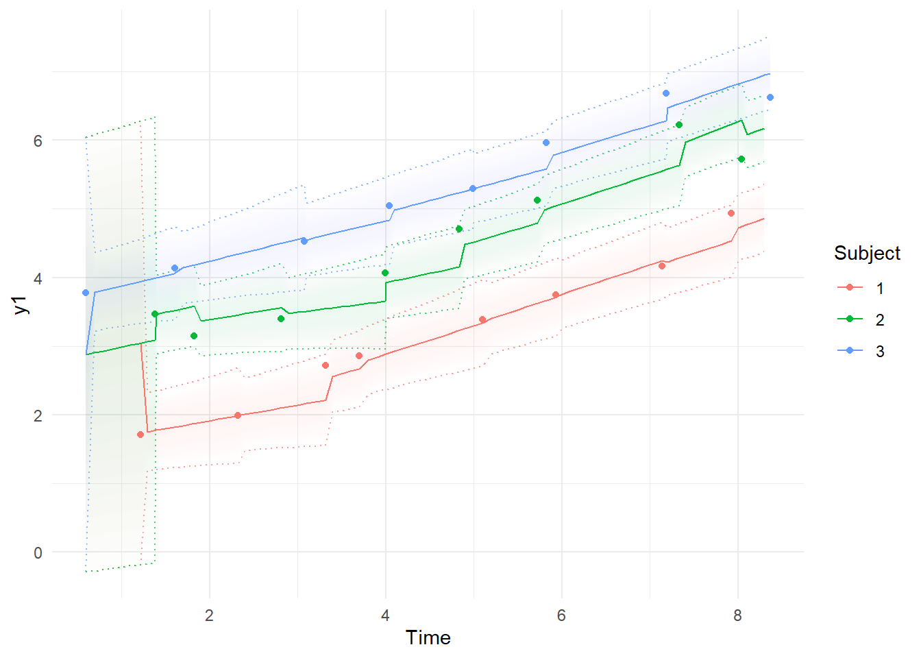
ctKalman(fit,plot=TRUE, #predicted (conditioned on past time points) observation values.
  kalmanvec=c('y','yprior'),
  subjects=1:3, timestep=.1) 

ctKalman(fit,plot=TRUE, #smoothed (conditioned on all time points) observation values.
  kalmanvec=c('y','ysmooth'),subjects=1:3,timestep=.1 )

Note the differences between the first plot, using the Kalman filter predictions for each point, where the model simply extrapolates forwards in time and has to make sudden updates as new information arrives, and the smoothed estimates, which are conditional on all time points in the data – past, present, and future. In the first plot, it’s possible to see the system slowly learning the intercept and slope parameters as more data arrives, and in the second, we see the corrections to the predictions based on the knowledge given by all the observations. These plots are based on the maximum likelihood estimate / posterior mean of the parameters.

Multivariate

Let’s look at a case with 2 latent processes, one of which has multiple indicators.

First, we generate some new data:

dat$eta2 <- dat$eta1 - .1*dat$time + rnorm(nrow(dat),0,.5)
dat$y2 <- dat$eta2 + rnorm(nrow(dat))
dat$y3 <- dat$eta2 + rnorm(nrow(dat),0,.2) + 3

Our new model looks like:

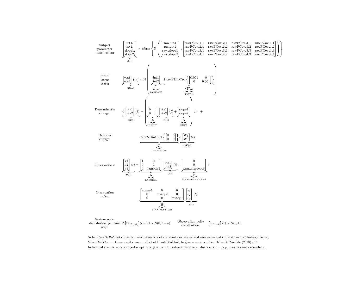
model <- ctModel(type='stanct', # use 'standt' for a discrete time setup
  DRIFT=0, #change doesn't depend on latent state
  DIFFUSION=0, #no random change in latent state
  CINT=c('slope1','slope2'), #freely estimated slopes
  T0MEANS=c('int1','int2'),
  MANIFESTMEANS=c(
    0,0,'manintercept3||FALSE'), #manifest intercepts with 1 free param, no individual variation.
  manifestNames=c('y1','y2','y3'),
  latentNames=c('eta1','eta2'),
  LAMBDA=c( #vector input interpreted column wise
    1,0,
    0,1,
    0,'lambda3') #Factor loading matrix, now with free param
    )

ctModelLatex(model,linearise = TRUE) #requires latex install -- will prompt with instructions in any case

In this case, the ctsem default of correlated individual differences for all intercept style parameters is more relaxed than we want (though there may be good reasons for allowing individual differences here!) and we have used the separator | notation to turn off individual variation on the manifest intercept parameter.

We fit the new model to the data…

fit<- ctStanFit(dat, model, optimize=TRUE, nopriors=TRUE, cores=2) 

and take a look at our new results:

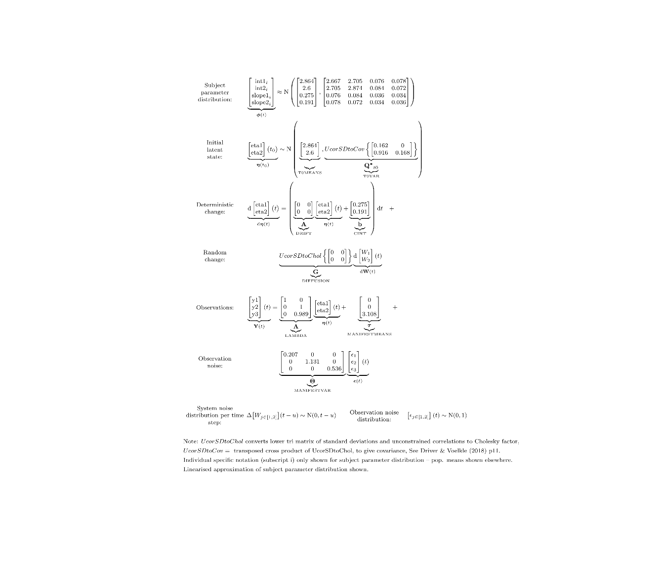
ctModelLatex(fit) #requires latex install -- will prompt with instructions in any case

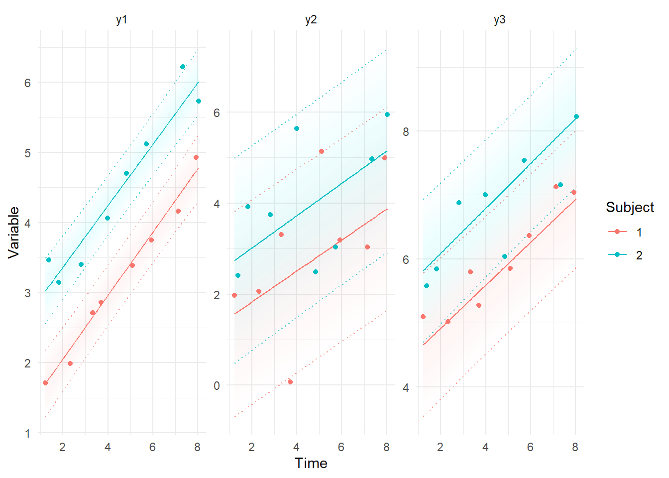
ctKalman(fit,plot=TRUE, #smoothed (conditioned on all time points) predictions.
  kalmanvec=c('y','ysmooth'),subjects=1:2,timestep=.1 ) 

State dependent measurement error

Ok, now let’s consider something that regular SEM can’t handle. What if our measurement instruments only work well for certain values of the latent variable?

Modify the data so measurement error depends on the latent state, eta.

dat$y1 <- dat$eta1 + 
  rnorm(nrow(dat),0, log1p(exp(.8*dat$eta1-3))) #add some state dependent noise
plot(dat$eta1,log1p(exp(.8*dat$eta1-3))) #plot measurement error sd against latent

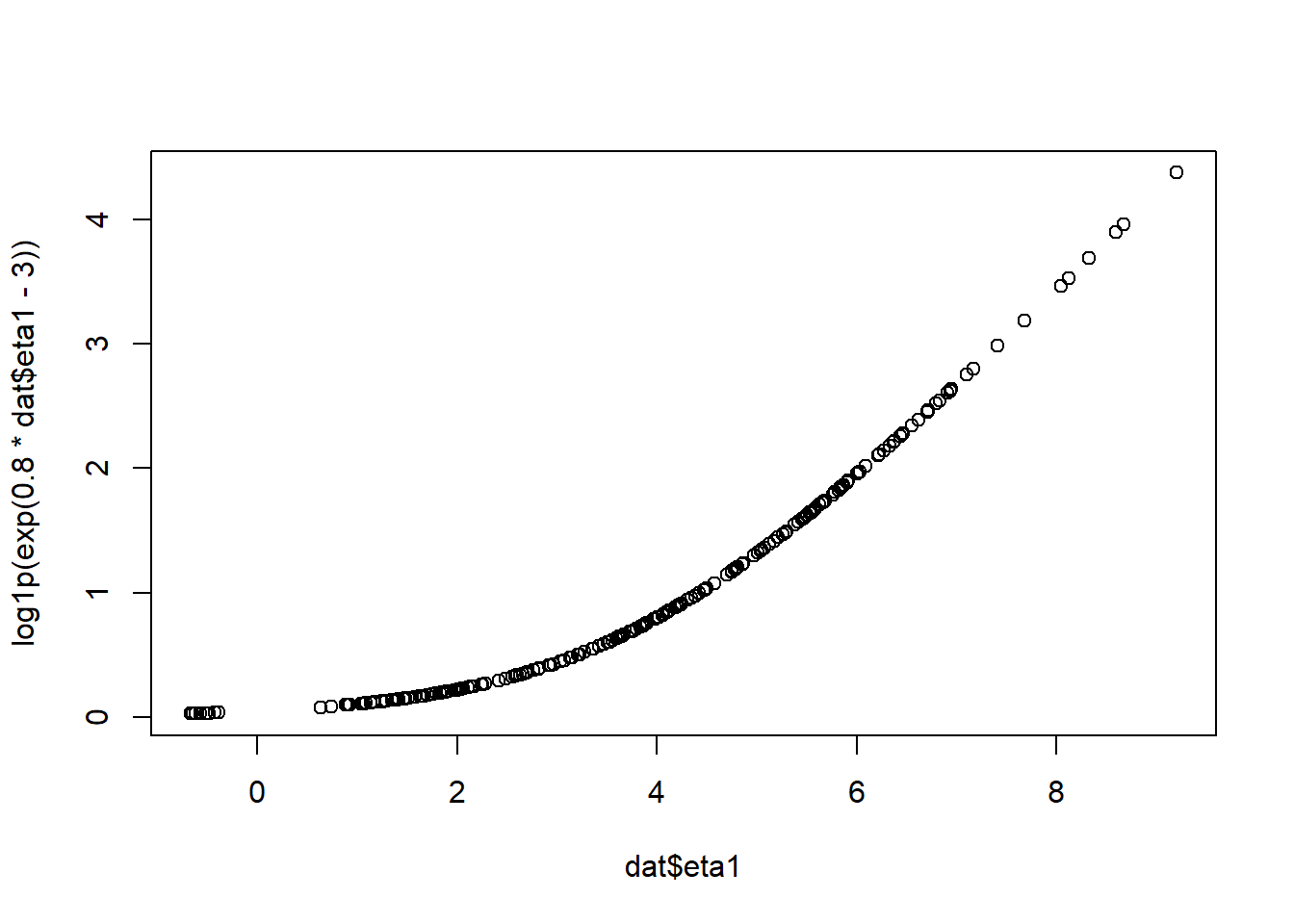
Include a dependency on eta1 in the MANIFESTVAR (measurement error) matrix, ensuring the results is always positive by using the log1p_exp (softplus) function, and making sure ctsem knows which are the free parameters in the complex parameter construction.

model <- ctModel(type='stanct', 
  DRIFT=0,
  DIFFUSION=0,
  CINT='slope',
  MANIFESTMEANS=0,
  manifestNames='y1',latentNames='eta1',
  LAMBDA=1,
  MANIFESTVAR='log1p_exp(errorsd_intercept + errorsd_byeta1 * eta1)', #complex sd parameter
  PARS=c('errorsd_intercept', 
    'errorsd_byeta1') #specify any free parameters within complex parameters
)

ctModelLatex(model) #requires latex install -- will prompt with instructions in any case

fit<- ctStanFit(dat, model)

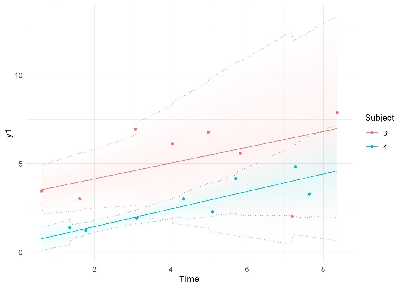
Now we can see that when the process has lower values, we are more certain about the model predictions because of reduced measurement error.

k=ctKalman(fit,plot=TRUE, #smoothed (conditioned on all time points) observation values.
  kalmanvec=c('y','ysmooth'),subjects=c(3,4))