ctsem is R software for statistical modelling using hierarchical state space models, of discrete or continuous time formulations, with possible non-linearities (ie state / time dependence) in the parameters. This is a super brief demo to show the basic intuition for Kalman filtering / smoother, and missing data imputation – for a quick start see https://cdriver.netlify.com/post/ctsem-quick-start/ , and for more details see the current manual at https://github.com/cdriveraus/ctsem/raw/master/vignettes/hierarchicalmanual.pdf

Data

Lets load ctsem (if you haven’t installed it see the quick start post!), generate some data from a simple discrete time model, and create some artificial missingness:

set.seed(3)
library(ctsem)

y <- 6 #start value
n <- 40 #number of obs
for(i in 2:n){ 
  y[i] = .9 * y[i-1] + .1 + rnorm(1,0,.5) # ar * y + intercept + system noise
}
y=y+rnorm(n,0,.2) #add measurement error
y=data.frame(id=1,y=y,time=1:n) #create a data.frame for ctsem

missings <- c(5,17:19,26,35) #a few random observations...

ymissings=y #save the missings to check later
ymissings$y[-missings]<-NA

y$y[missings]<-NA #remove the selected obs from our analysis data set

head(y)
##   id        y time
## 1  1 6.158752    1
## 2  1 5.176335    2
## 3  1 4.408774    3
## 4  1 4.592951    4
## 5  1       NA    5
## 6  1 3.284191    6

Model

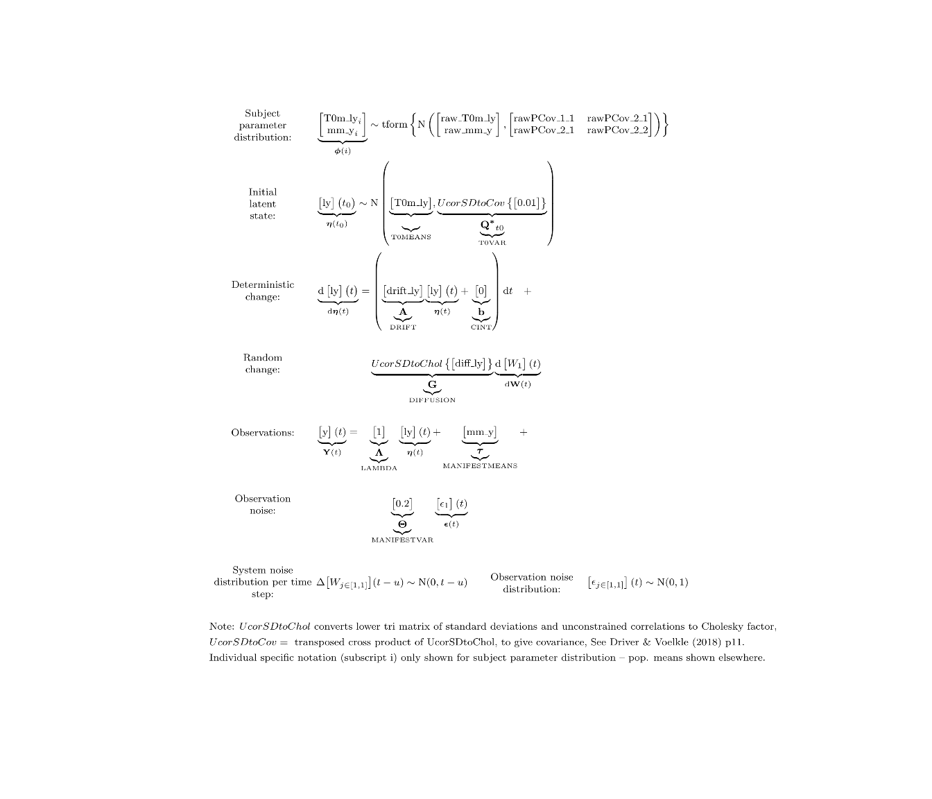
If we’re going to impute missing data, we need some kind of model for the imputation. The default model in ctsem is a first order auto / cross regressive style model, in either discrete or continuous time. There is correlated system noise, and uncorrelated measurement error. When multiple subjects are specified, the default is to have random (subject specific) initial states and measurement intercepts (with correlation between the two). For our purposes here, we’re going to rely mostly on the defaults, and use a continuous time, differential equation format – the discrete time form would also work fine for these purposes, but visualising the difference between the filter and smoother is much more obvious with the continuous time approach. Besides the defaults, we also fix the initial latent variance to a very low value (because we only have one subject), and the measurement error variance (because having system and measurement noise makes for better visuals but we can’t easily estimate both with so little data).

model <- ctModel(type='stanct', # use 'standt' for a discrete time setup
  manifestNames='y',latentNames='ly',
  T0VAR=.01, #only one subject, must fix starting variance
  MANIFESTVAR=.2, #fixed measurement error, not easy to estimate with such limited data
  LAMBDA=1) #Factor loading fixed to 1
 
ctModelLatex(model) #requires latex install -- will prompt with instructions in any case

Fit using optimization and maximum likelihood:

fit<- ctStanFit(y, model, optimize=TRUE, nopriors=TRUE, cores=2)

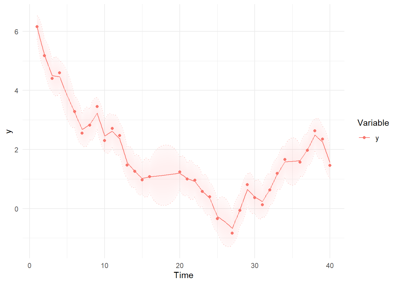
Then we can use summary and plotting functions. Note the differences between the first plot, using the Kalman filter predictions for each point, where the model simply extrapolates forwards in time and has to make sudden updates as new information arrives, and the smoothed estimates, which are conditional on all time points in the data – past, present, and future. These plots are based on the maximum likelihood estimate / posterior mean of the parameters.

summary(fit)

kp<-ctKalman(fit,plot=TRUE, #predicted (conditioned on past time points) predictions.
  kalmanvec=c('y','yprior'),timestep=.1)

ks<-ctKalman(fit,plot=TRUE, #smoothed (conditioned on all time points) latent states.
  kalmanvec=c('y','ysmooth'),timestep=.1 )

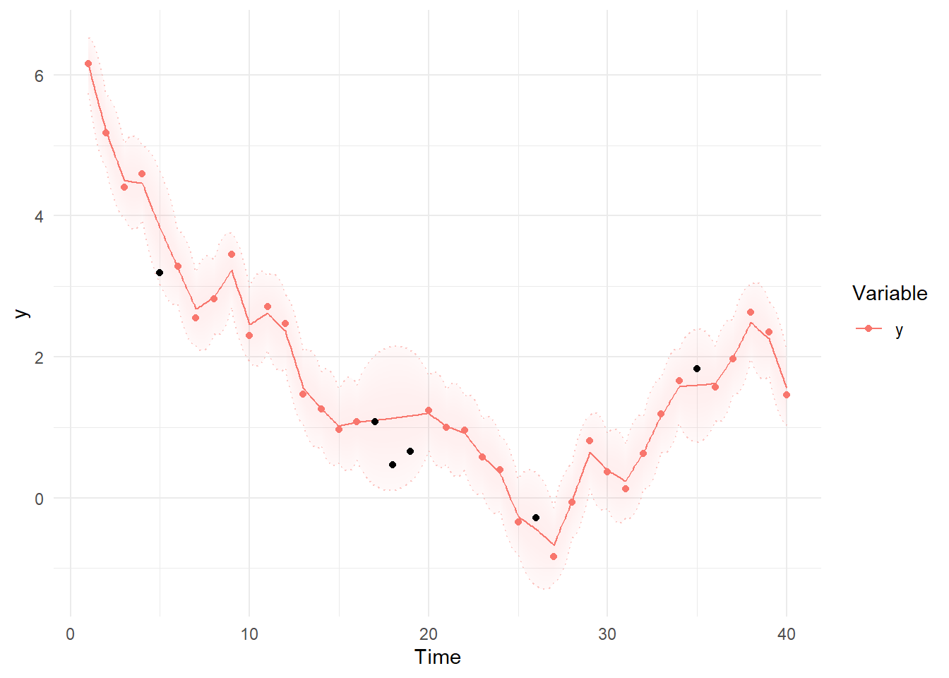
We can modify the ggplot objects we created to include the data we dropped:

library(ggplot2)
kp= kp + geom_point(data = data.frame(Variable='y', Value=ymissings$y,
    Element='y',Time=ymissings$time), col='black')
plot(kp)

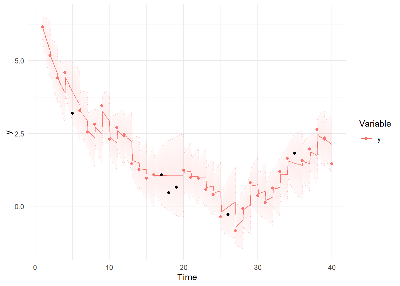
ks= ks + geom_point(data = data.frame(Variable='y', Value=ymissings$y,
    Element='y',Time=ymissings$time), col='black')
plot(ks)

To access the imputed, smoothed values without plotting directly, we use the mean of our parameter samples to calculate various state and observation expectations using the ctStanKalman function. (In this case the samples are based on the Hessian at the max likelihood, but they could potentially come via importance sampling or Stan’s dynamic HMC if we used different fitting options.) If we wanted more or different values to be available from such an approach, the easiest way is to include them as missing observations in the dataset used for fitting.

k<-ctStanKalman(fit,collapsefunc = mean) 
str(k$ysmooth) 
k$ysmooth[1,missings,]