Accelerated Longitudinal and Multiple Group Designs in ctsem

Generate some data

Here we specify a single latent process of state dependent growth over time, where individuals also exhibit stable differences over time, and cohort differences are found in both the amount of measurement error, and the amount of state dependency in growth. Such cohort differences could be due to genuine differences between the true underlying process of each group, as in this case, but it’s important to keep in mind that any heterogeneity could also come about due to model limitations. To imagine the latter case, one need only consider multiple age groups, all subject to quadratic growth, but fit with a linear growth model as the baseline – each group will then be estimated with a different linear slope, and if the number of age groups was high enough we could approximately recover the true quadratic trend.

Anyway, on to the data generation, though you might want to skip this code!

set.seed(1)
library(ctsem)


measurementErrorSD <- c(1, .5, .2, .2) #different cohorts measurement error
drift <- c(-.3, -.5, -.6, -.6) 

for(cohorti in 1:4){
  
  gm <- ctModel(
    LAMBDA=diag(1), #single observed variable and single process
    Tpoints = 50,
    CINT=5,
    TRAITVAR=diag(1), #include individual differences in continuous intercept
    DRIFT=drift[cohorti], #temporal dynamics
    DIFFUSION=.5,
    MANIFESTVAR=0) #measurement error sd fixed to zero so we can plot true scores
  
  #when generating data, free pars are set to 0
  d <- data.frame(ctGenerate(ctmodelobj = gm,n.subjects = 50,
    burnin = 5,dtmean = .1),Cohort2=0,Cohort3=0,Cohort4=0, Cohort=cohorti)
  d$id <- paste0('Cohort',cohorti,'_id',d$id)
  
  d <- d[d$time < (cohorti) & d$time > (cohorti-1),]
  
  d$Yobs <- d$Y1 + rnorm(nrow(d),0,measurementErrorSD[cohorti]) #add measurement error
  
  if(cohorti == 1){
    dat <- d
  } else{
    d[[paste0('Cohort',cohorti)]] <- 1 #if other than first (baseline) cohort, set appropriate dummy
    dat <- rbind(dat,d)
  }
}

Let’s take a look at our data:

library(ggplot2)

ggplot(dat, aes(y=Y1,x=time,colour=factor(Cohort),group=id))+
  geom_line()+theme_bw()+
  geom_line(mapping = aes(y=Yobs),alpha=.3)+
  guides(colour='none')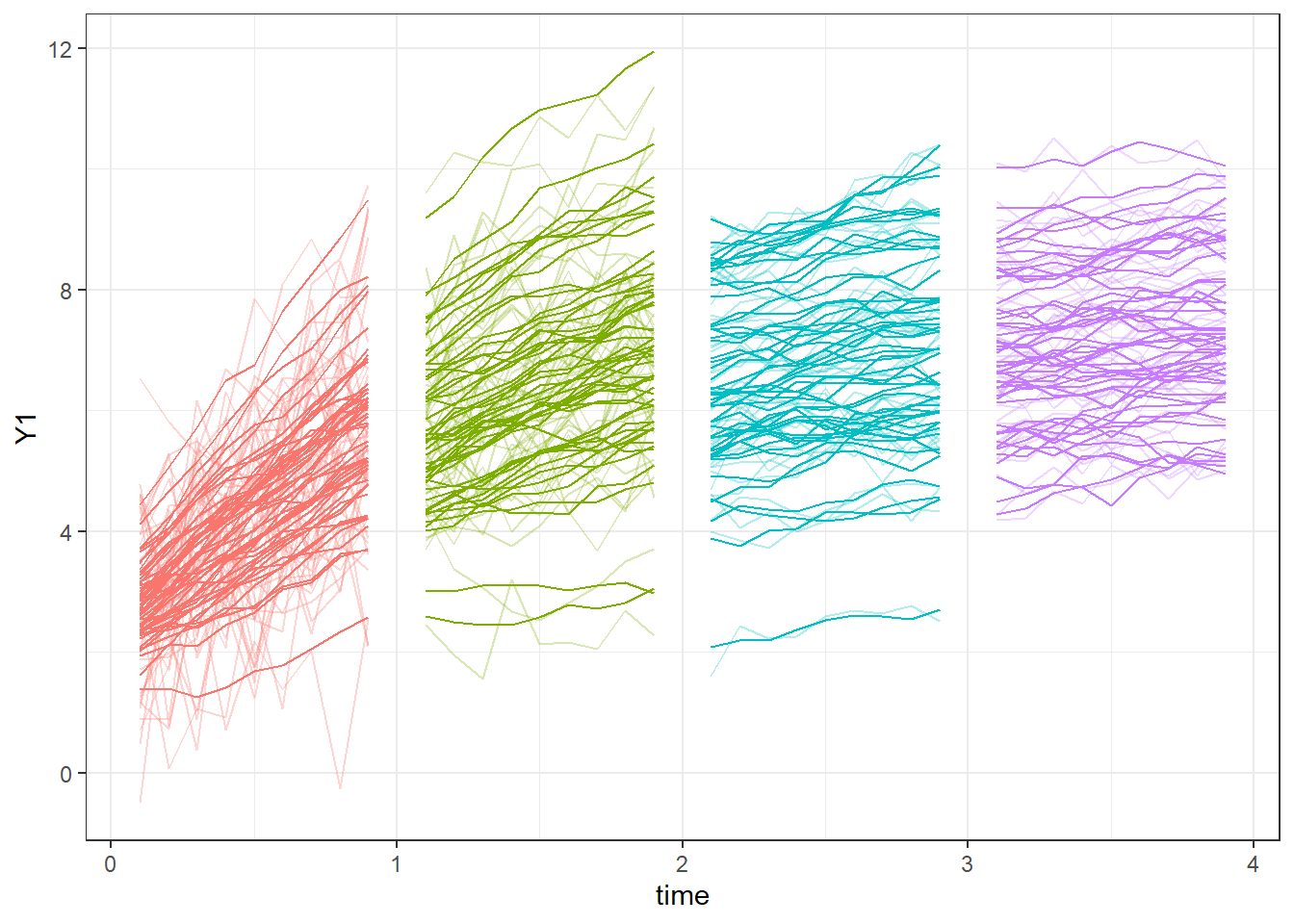

One aspect to modelling such accelerated designs with ctsem is how the first observation is handled. ctsem includes a vector called T0MEANS that specifies the starting point for all processes in the system, and this starting point is assumed to apply to the time of first observation for each subject. In this sense a better name for the vector would have been INITIALMEANS, but hindsight is harsh in software development sometimes. In any modelling where the T0MEANS parameters should apply to a specific point in time rather than simply whenever the first observation was made, we need to make sure that each individual has a first observation at the time of interest, even if all observed variables are NA. So we do this here, setting every subject to have an observation at the earliest age in the sample:

dat0 <- dat[!duplicated(dat$id),] #create extra dataframe containing one observation of each subject
dat0$time <- min(dat$time) #set the times of each observation to the time of earliest observation in our dataset
dat0$Y1 <- dat0$Yobs <- NA #set observed variables to NA (but keep the info for time independent predictors such as group dummies!)
dat <- merge(dat, dat0, all = TRUE)

We can set up and fit a baseline model that does not account for cohort differences. For the most part we rely on the model defaults, which is to have freely estimated temporal effects (DRIFT) and temporal fluctuations (DIFFUSION) matrices, as well as stable individual differences in the starting point (T0MEANS) and any other freely estimated intercept parameters. Since we are dealing with growth over time it is usually clearer to use the ‘continuous’ intercept (CINT, affecting the latent processes) to capture the linear slope effect and fix MANIFESTMEANS (intercept on the measurement equation) to zero. Since we just have one observed variable and only want to model one latent process, the factor loading matrix LAMBDA is simply a 1x1 matrix of 1.

m1 <- ctModel(
  type='stanct',
  CINT='cint', 
  MANIFESTMEANS = 0,
  LAMBDA=diag(1),
  manifestNames = 'Yobs')

f1 <- ctStanFit(datalong = dat, ctstanmodel = m1, cores=2)

To include cohort information, we take our first cohort as the baseline group, then add a dummy covariate for each subsequent cohort to the time independent predictors – these moderate all of the individual system parameters by default, but do not moderate the standard deviation or correlation structure of any random effects individual differences.

m2 <- ctModel(
  type='stanct',
  CINT='cint', 
  TIpredNames = c('Cohort2','Cohort3','Cohort4'),
  MANIFESTMEANS = 0,
  LAMBDA=diag(1),
  manifestNames = 'Yobs')

#ctModelLatex(m2) #view the full model as a pdf

f2 <- ctStanFit(datalong = dat, ctstanmodel = m2, cores=2)

With cohort influences on the system parameters, the model looks like:

knitr::include_graphics('mdefaulttex.png')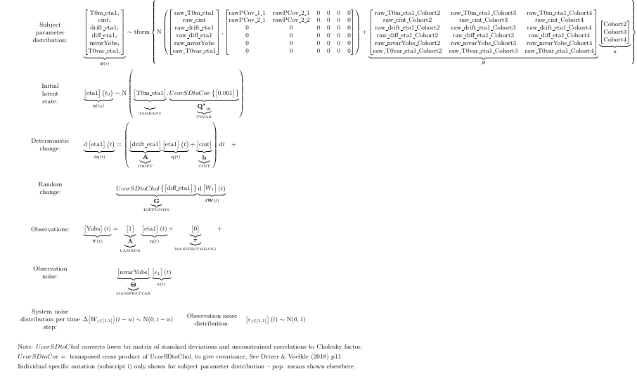

We can plot expectations for a subject from each group based only on covariates (i.e. group membership) as follows.

plot<-ctKalman(f2, subjects = dat$id[!duplicated(dat$Cohort)], plot=T, 
  kalmanvec=c('yprior'),removeObs = T, polygonsteps=1)
print(plot+facet_wrap(vars(Subject)))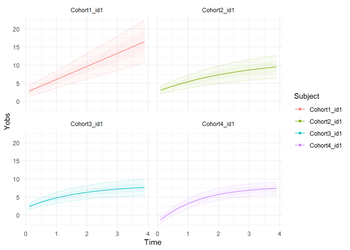

Or if we want to display the best estimate for each individuals trajectory, conditioning on all available information (so no these are not forward predictions), we use the Kalman ‘smoothed’ estimates, like so:

ctKalman(f2, subjects = dat$id[!duplicated(dat$Cohort)], plot=T, 
  kalmanvec=c('y','etasmooth'),facets=NA)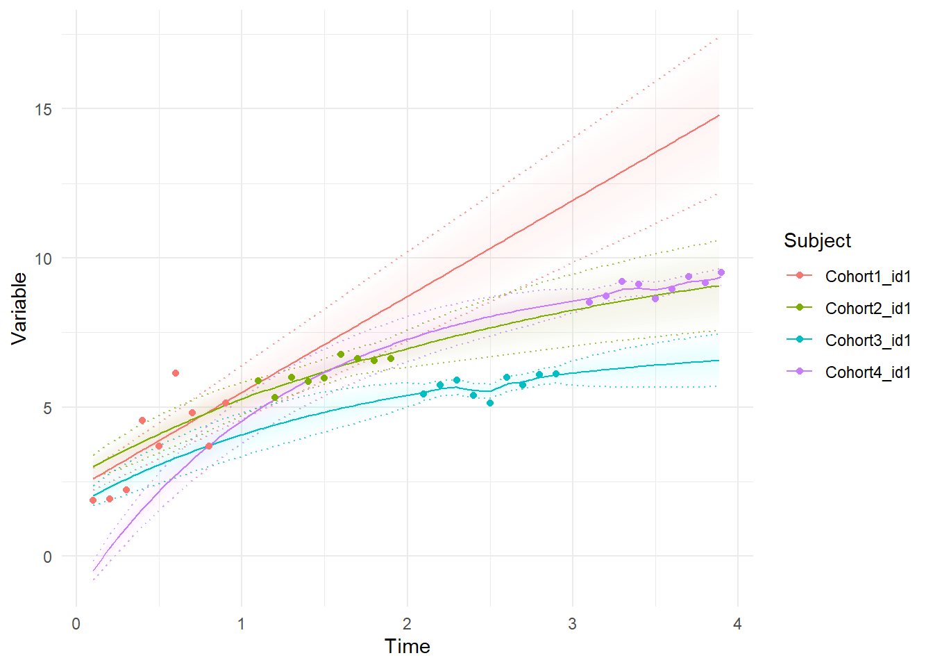

If cohort effects on the parameter means is deemed insufficient, and group differences on the random effects structure of parameters is also desirable, then for the time being at least you can’t rely on ctsem’s automatic random effects structuring, but have to build your own by extending the number of system states, and disabling ctsem’s random effects. System states for stable individual differences are essentially an unchanging process with a freely estimated starting point (T0MEANS), and freely estimated covariance with other processes at the start point (T0VAR).

m3 <- ctModel(
  type='stanct',
  manifestNames = 'Yobs',
  latentNames=c('eta','intercept'), #we now have two processes -- main process eta, and extra process 'intercept'
  CINT=0, #we no longer estimate a parameter here, because we have moved it to the 2nd system process
  DRIFT=c( 
    'drift1', 1, #self feedback parameter, and effect of intercept process on main process fixed to 1
    0, 0), #no effect of main process on intercept, and intercept process does not change so auto effect is 0
  DIFFUSION=c(
    'diffusion1',0, #only the main process is subject to random fluctuations
    0,0), 
  T0VAR=c( #since we are now specifying individual differences by manually extending the system matrices, 
    't0v11',0, #stable individual differences come in via the initial variance (t0var) in starting points. 
    't0v21','t0v22'), #correlation parameters are specified in the lower off diagonal.
  T0MEANS=c(
    't0eta||FALSE', #freely estimate starting points for both processes but,
    't0intercept||FALSE'), # *disable* ctsem's random effects handling (set to FALSE)
  TIpredNames = c('Cohort2','Cohort3','Cohort4'),
  MANIFESTMEANS = 0,
  LAMBDA=matrix(c(1,0),nrow=1, ncol=2)) #intercept process does not directly affect observed variables)

f3 <- ctStanFit(datalong = dat, ctstanmodel = m3, cores=2)

In this case, we can also use the plot functions to observe how the estimates of the random effects individual differences get updated with each point of new data – before any of an individuals observations are known, the estimate is simply the mean for the cohort, but once observations start coming in, the prediction for individuals continuous intercept gets updated, just like the forward predictions for the main latent process of interest, eta. These plots are from the kalman predictions, which are requested by specifying either ‘etaprior’ (for latent process) or ‘yprior’ (for observation level) predictions.

ctKalman(f3, subjects = dat$id[!duplicated(dat$Cohort)],plot=T,kalmanvec='etaprior')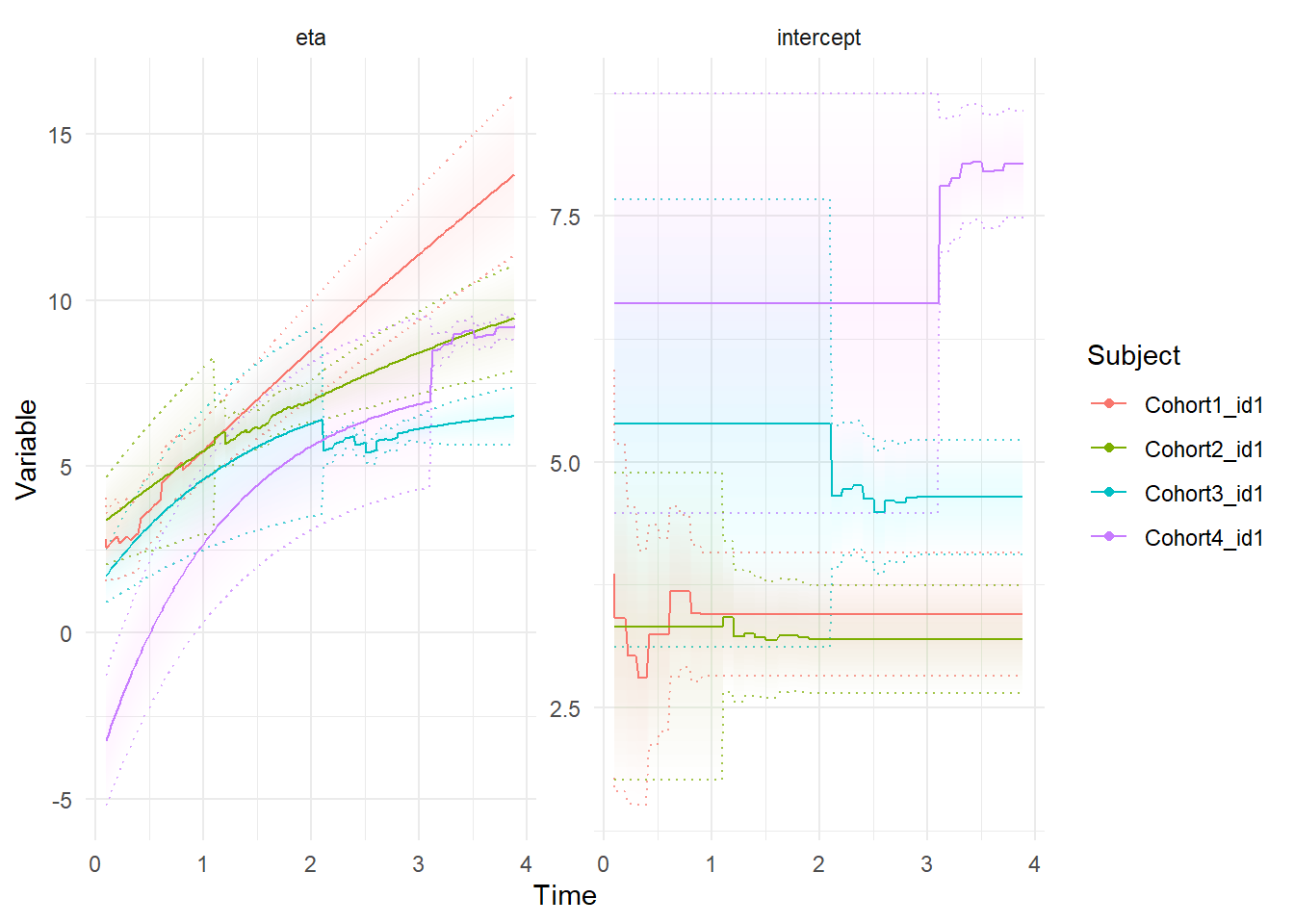

We can compare the different models for cohort differences using a few different approaches.

Either AIC, with lower being better:

print(data.frame(
  Model=c('m1','m2','m3'),
  AIC=c(summary(f1)$aic, summary(f2)$aic, summary(f3)$aic)))
##   Model      AIC
## 1    m1 4081.966
## 2    m2 3053.313
## 3    m3 3070.998

Or using chi-square tests, where a low probability (e.g. < .05) indicates the more complex model is performing significantly better:

ctChisqTest(f2,f1)
## [1] 3.579979e-216
ctChisqTest(f3,f2)
## [1] 0.9999959

Or using cross validation, to quantify prediction performance on out of sample data. The default is 10 fold cross validation, where 10% of subjects are dropped during parameter estimation for each of 10 fits, and the ‘out of sample’ log likelihood is based on the sum of log likelihoods over these 10 groups. Higher likelihoods indicate better models.

l1=ctLOO(f1,cores=1)
l2=ctLOO(f2,cores=1)
l3=ctLOO(f3,cores=1)

print(data.frame(
  Model=c('m1','m2','m3'),
  CV10FoldLogLik=c(l1$outsampleLogLik,l2$outsampleLogLik,l3$outsampleLogLik)))
##   Model CV10FoldLogLik
## 1    m1      -2045.691
## 2    m2      -1525.703
## 3    m3      -1534.040

In this case, the cohort differences model where only the means differ, and random effects distributions are otherwise the same, is the most effective model. This is consistent with how the data were generated.