ctsem is R software for statistical modelling using hierarchical state space models, of discrete or continuous time formulations, with possible non-linearities in the parameters. In this post I’ll walk through some of the basics of ctsem usage, for more details see the current manual at https://github.com/cdriveraus/ctsem/raw/master/vignettes/hierarchicalmanual.pdf

Installation and loading of ctsem

Within R, for the CRAN version of ctsem simply run:

install.packages('ctsem') 

Or for the github version, with extra setup for stan that may be useful if stan is not installed:

source(file = 'https://github.com/cdriveraus/ctsem/raw/master/installctsem.R')

library(ctsem)

This should work reliably for most / all cases – occasionally the rstan installation does not work smoothly, and errors can occur when models that require compilation (more complex models) are specified. In such cases, the ctsem github page https://github.com/cdriveraus/ctsem offers some remedies, the Stan forum is very helpful https://discourse.mc-stan.org/, or you can get in touch with me…

Data

ctsem uses long format data, requires time and id columns, as well as at least one indicator / manifest variable. For this example we will use the sunspots dataset provided within R, and setup a damped linear oscillator.

ssdat <- data.frame(id=1, 
  time=do.call(seq,as.list(attributes(sunspot.year)$tsp)), 
  sunspots=sunspot.year)

head(ssdat)
##   id time sunspots
## 1  1 1700        5
## 2  1 1701       11
## 3  1 1702       16
## 4  1 1703       23
## 5  1 1704       36
## 6  1 1705       58

Model

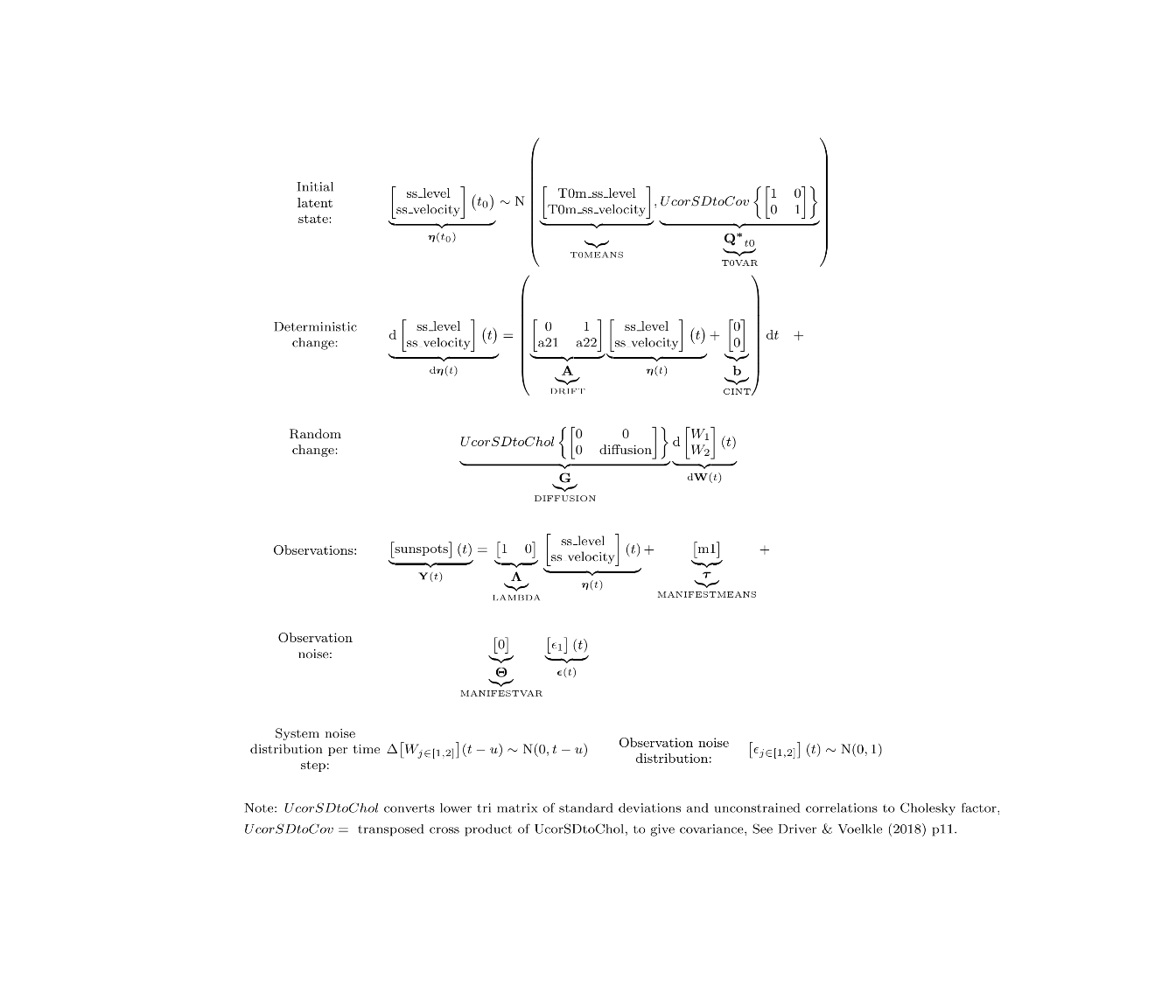
To fit a model using ctsem, the model is first specified using the ctModel function, then fit using the ctStanFit function. Free parameters are specified as strings, fixed values as numerics. Different slots of the matrices have different constraints by default, for DRIFT[2,1] we restrict the effect of sunspot level on sunspot velocity (parameter a21) to be negative by specifying a custom transformation in the 2nd slot, using the | symbol to separate slots. We also explicitly disallow any parameter variation across subjects, although since we have only 1 subject here this would have occurred anyway during fitting.

ssmodel <- ctModel(type='stanct',
  manifestNames='sunspots',
  latentNames=c('ss_level','ss_velocity'),
  LAMBDA=c( 1, 0),
  DRIFT=c(0, 1,
  'a21 | -log1p(exp(-param))-1e-5', 'a22'),
  MANIFESTMEANS=c('m1'),
  MANIFESTVAR=0,
  T0VAR=diag(1,2), #init variance, would have been fixed automatically since only 1 subject
  CINT=0,
  DIFFUSION=c(0, 0,
  0, "diffusion"))

ssmodel$pars$indvarying <- FALSE #set all pars to fixed across subjects (also automatic in this case)
  
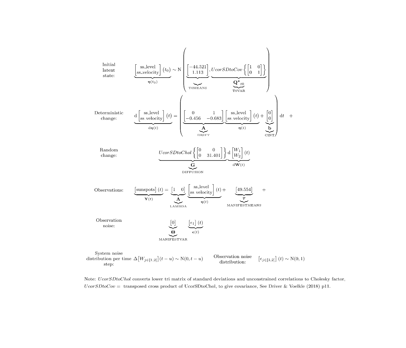
ctModelLatex(ssmodel)

Fit using maximum likelihood:

ssfit <- ctStanFit(ssdat, ssmodel, cores=2)

Then we can use summary and plotting functions:

summary(ssfit)

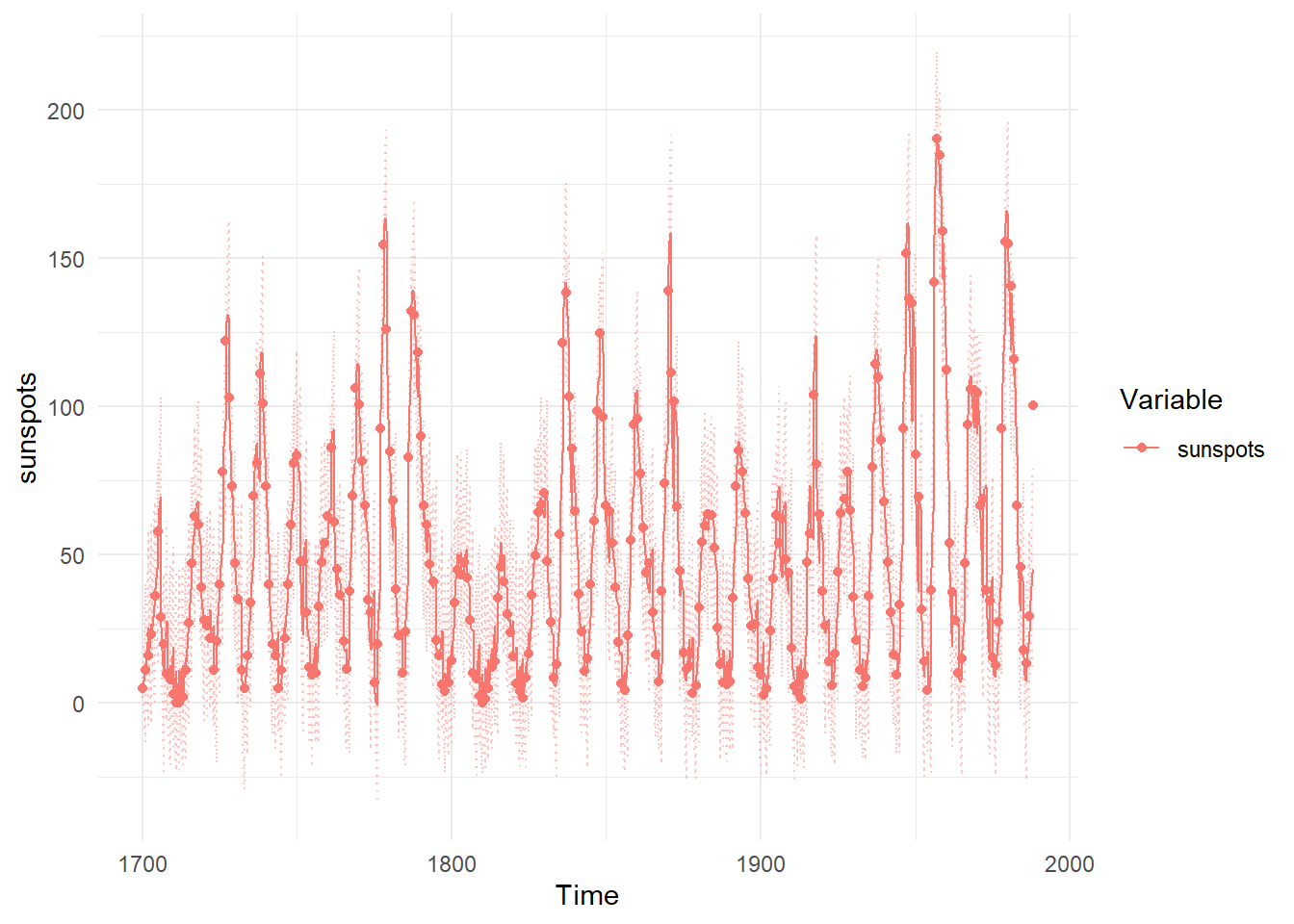
ctKalman(ssfit,plot=TRUE, #predicted (conditioned on past time points) predictions.
  kalmanvec=c('y','yprior'), timestep=.1)

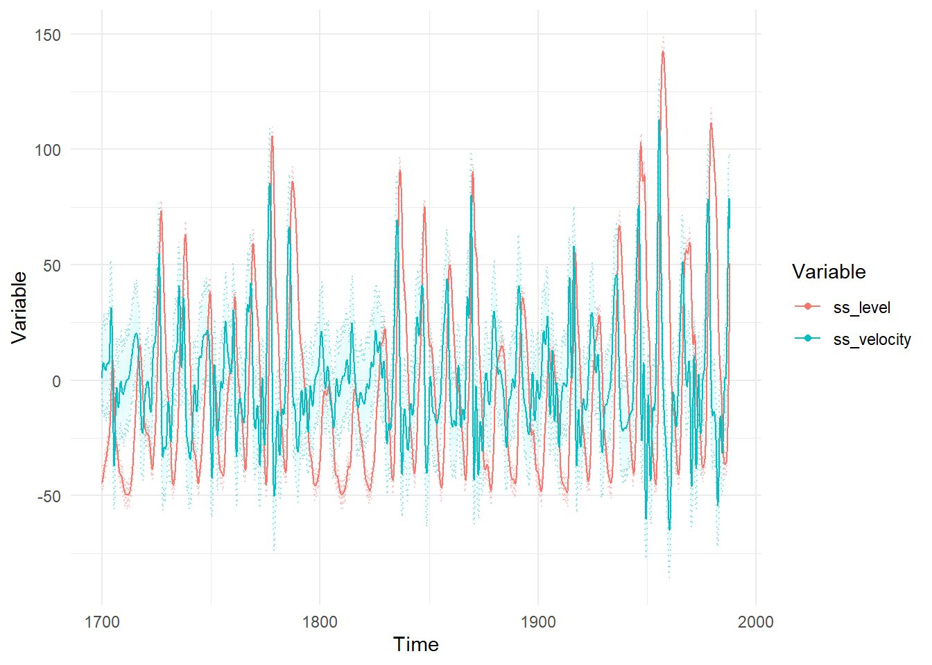
ctKalman(ssfit,plot=TRUE, #smoothed (conditioned on all time points) latent states.
  kalmanvec=c('etasmooth'), timestep=.1)

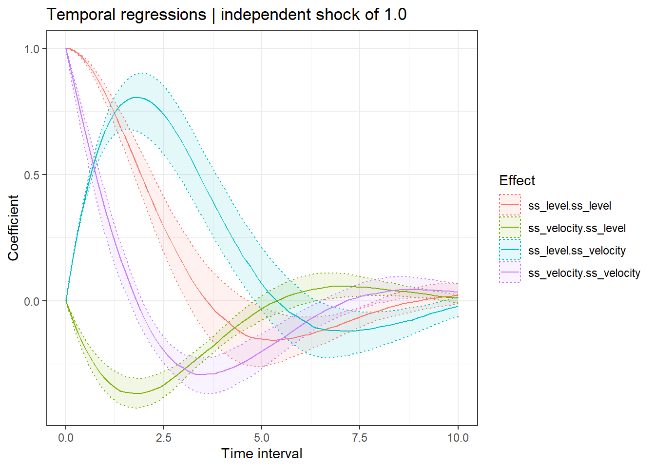
ctStanDiscretePars(ssfit,plot=TRUE) #impulse response

ctModelLatex(ssfit)

To fit using a Bayesian approach, we need to pay more attention to our transformations / priors:

plot(ssmodel)

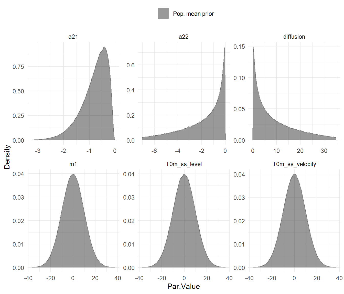
Even though we only have one subject for this case, the model doesn’t know that until we fit it to data, and by default intercept style parameters are allowed to vary across subjects – hence the blue and red plots showing possible distributions of subject parameters conditional on a mean of 1 standard deviation less or more.

Most priors should be workable, but since the ctsem defaults are designed for data centered around zero, the manifest means parameter will need the prior adjusted. At the same time we may as well disable individual variation, possible either by using the 3rd parameter slot (with | separators) or by modifying the object directly after specification. Both approaches are shown here:

ssmodel <- ctModel(type='stanct',
  manifestNames='sunspots',
  latentNames=c('ss_level', 'ss_velocity'),
  LAMBDA=c( 1, 0),
  T0MEANS=c('t0_sslevel||FALSE', 't0_ssvelocity||FALSE'),
  DRIFT=c(0, 1,
  'a21 | -log1p(exp(-param))-1e-5','a22'),
  MANIFESTMEANS=c('m1|param*10+44'),
  MANIFESTVAR='merror',
  T0VAR=diag(1e-3,2), #this would have been set automatically since only 1 subject
  CINT=0,
  DIFFUSION=c(0, 0,
  0, "diffusion"))

ssmodel$pars$indvarying <- FALSE

Looking at the MANIFESTMEANS specification, we’ve used the second slot (via | separator) to modify the prior / transformation. param*10+44 implies that param, a standard normal parameter, is multiplied by 10 and offset by +44, to give a normal distribution centered at 44 with a standard deviation of 10.

We can use the functions of ctsem to generate data from our prior distribution, according to the structure (i.e. the timing of observations and any covariates) specified in our data, then use this to create a prior predictive plot – comparing samples of possible trajectories from the prior distribution to our actual data:

library(ggplot2)
priorpred <- ctStanGenerate(cts = ssmodel, 
  datastruct = ssdat, cores=2, nsamples = 200)

ggplot(data=ssdat,mapping = aes(y=sunspots,x=time)) + 
  theme_minimal()+
  geom_line(data=data.frame(sunspots=c(priorpred$Y),
    time=rep(ssdat$time,dim(priorpred$Y)[1]),
    sample=factor(rep(1:dim(priorpred$Y)[1],each=dim(priorpred$Y)[2]))), 
    alpha=.3,colour='red',aes(group=sample))+
  geom_line(colour='black',size=1)+
  coord_cartesian(ylim = c(-100,200))

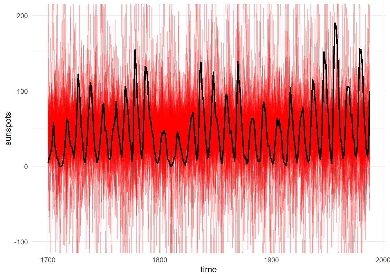
Since this doesn’t look obviously unreasonable, we’ll go ahead and fit using Stan’s Hamiltonian Monte Carlo and plot the posterior distributions of parameters:

ssfit <- ctStanFit(ssdat, ssmodel, 
  iter=300, chains=2, cores=2,optimize=FALSE,nopriors=FALSE)

ctStanPlotPost(ssfit)

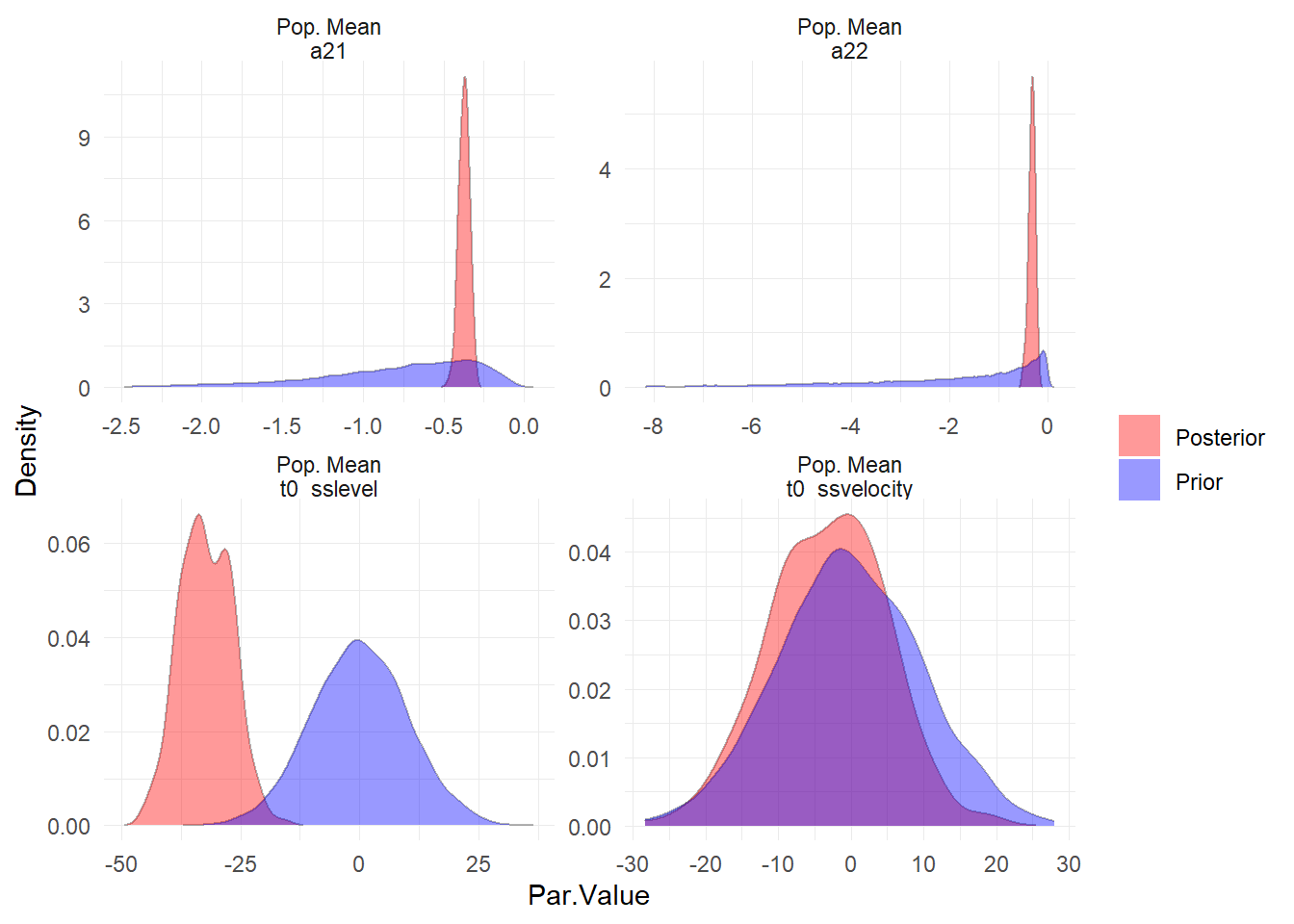
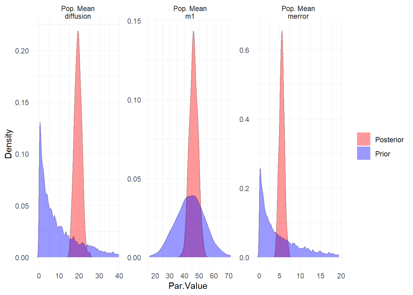
Evidently our priors on the starting points (t0) for the latent processes could have been better, but this should not have too large an impact on the model overall, given the length of the series.

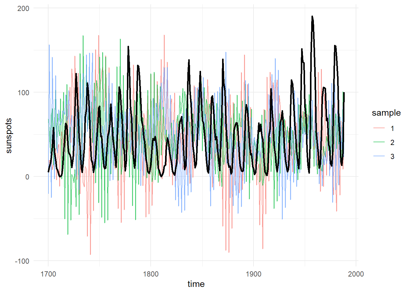
Given the model fit, we can also generate new data from the posterior, in the same structure (re missingness and covariates) as the original, then compare various quantities between the generated and the actual data. The following shows 3 samples of generated data (in colour) against the original (in black).

postpred <- ctStanGenerateFromFit(ssfit, fullposterior = TRUE, nsamples = 3)

ggplot(data=ssdat,mapping = aes(y=sunspots,x=time)) + 
  theme_minimal()+
  geom_line(data=data.frame(sunspots=c(postpred$generated$Y),
    sample = factor(rep(1:dim(postpred$generated$Y)[1],
      each=dim(postpred$generated$Y)[2])),
    time=rep(postpred$standata$time,dim(postpred$generated$Y)[1])), 
    alpha=.7,aes(colour=sample),size=.5)+
  geom_line(colour='black',size=1)