Discrete Time Models Using ctsem?

Model Specification

We specify a bivariate process model, with each process measured by a single (noisy) indicator (leaving out our second stress indicator for the time being). Intercepts (here, MANIFESTMEANS) and initial parameters (T0MEANS) default to indivdually varying, but we specify explicitly here in any case as a demonstration (using the | separator notation). In fact, we specify the entire model explicitly, while since most parameters here are freely estimated, we could have left it to ctsem defaults.

model <- ctModel(
  LAMBDA = diag(2), #factor loadings / measurement structure
  type = 'standt', #could also choose stanct for continuous time modelling.
  manifestNames = c('Stress','Quality'),
  latentNames = c('Stress','Quality'),
  T0MEANS = c('t0_stress','t0_quality'), #starting values for latent processes
  MANIFESTMEANS = c('mi_stress||TRUE','mi_quality||TRUE'), #intercepts on observed variables
  MANIFESTVAR = c( #vectors are coerced rowwise into matrices of the right shape, 2x2 in this case
    'merr_stress',0,
    0,'merr_quality'),
  DRIFT = c(  #temporal dependence matrix, autoregression on the diagonal, cross regression off diagonal
    'a11','a12',
    'a21','a22'),
  DIFFUSION = c( #system noise. sd's on diagonal, unconstrained correlations on lower triangle
    'diff11',0,
    'diff21','diff22'),
  CINT = 0 #single values are repeated as many times as necessary (here, twice, one for each process)
  )

#ctModelLatex(model) #view model in pdf (i.e. readable) form. Requires latex compiler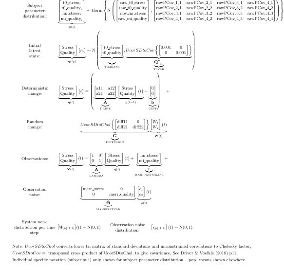

Model Fit and Plots

fit <- ctStanFit(datalong = dat,ctstanmodel = model, cores=2)

#ctModelLatex(fit) #view dynamic system estimates in equation form, requires latex compiler

ctKalman(fit,kalmanvec=c('y','yprior'),plot=TRUE, subjects=1:2) #forward predictions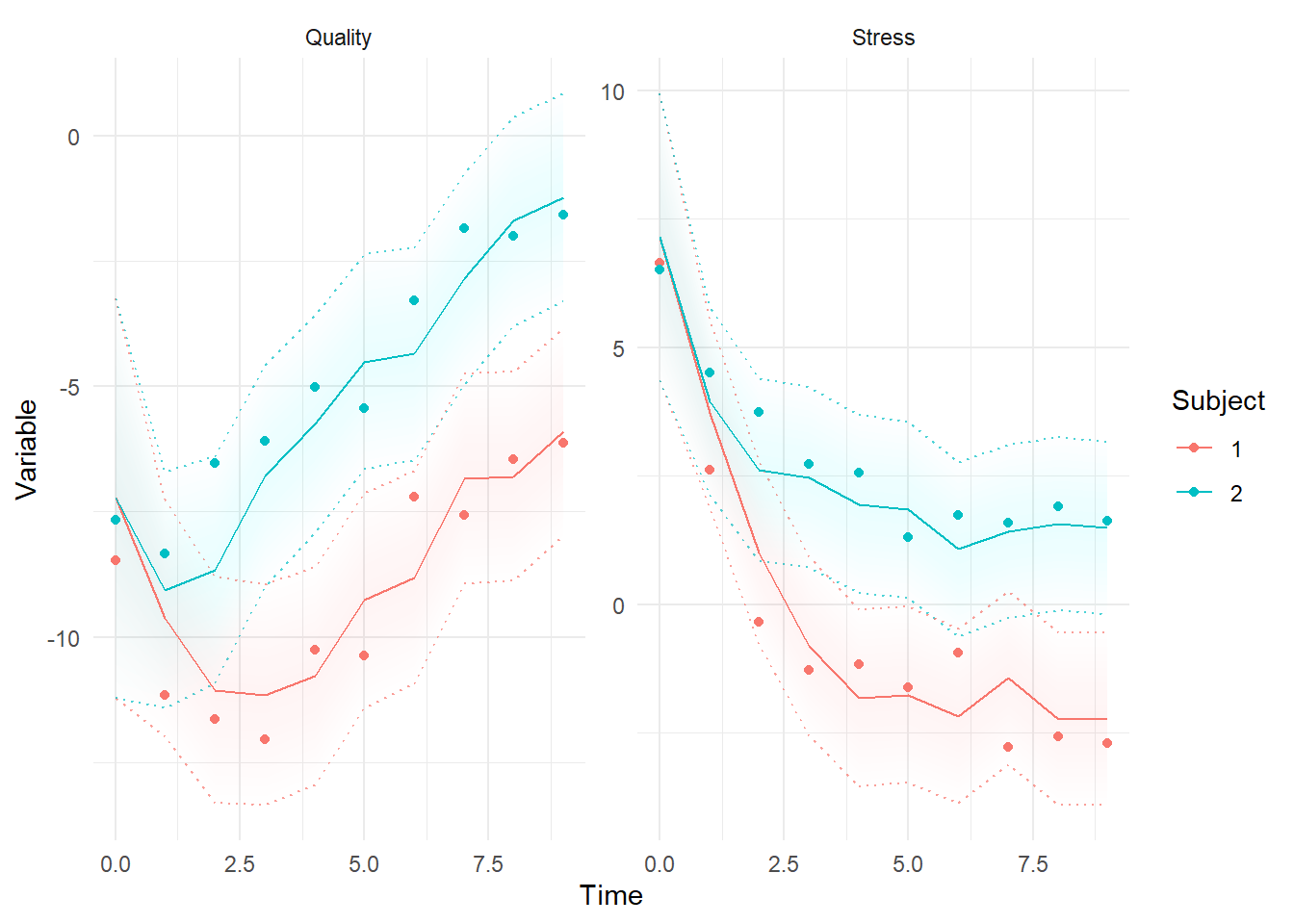

ctKalman(fit,kalmanvec=c('y','ysmooth'),plot=TRUE, subjects=1:2) #best estimates conditional on all data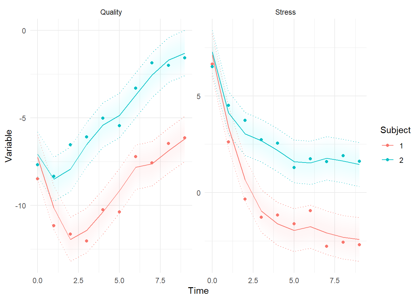

ctKalman(fit,kalmanvec=c('y','yprior'),plot=TRUE, subjects=1,removeObs = T) #predictions before seeing any data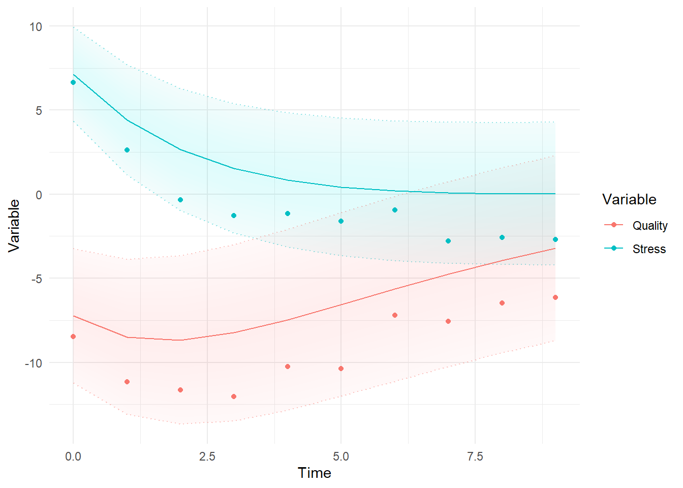

ctStanDiscretePars(fit,plot=T)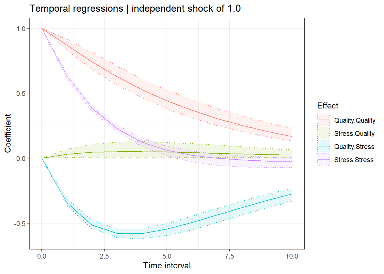

The previous plot shows the discrete-time regression coefficients for different lags – note that this is still a first order model (sometimes called lag 1), but because of the inclusion of measurement error and the possibility for missing data, higher lag effects are relevant. Put differently, the impact of a change at one point propagates further than the next observation, these plots show that propagation.

General summary information is found with the summary function, not shown here in full.

s <- summary(fit)
print(s$popmeans,digits=1) #basic system parameters
##               mean   sd   2.5%   50% 97.5%
## t0_stress     6.70 0.32  6.052  6.70  7.33
## t0_quality   -7.80 0.60 -8.933 -7.77 -6.67
## a11           0.63 0.01  0.612  0.63  0.65
## a12           0.03 0.02  0.004  0.03  0.06
## a21          -0.34 0.01 -0.367 -0.34 -0.31
## a22           0.87 0.02  0.829  0.87  0.91
## diff11        0.63 0.03  0.579  0.63  0.68
## diff21        1.00 0.00  1.000  1.00  1.00
## diff22        0.82 0.04  0.748  0.82  0.89
## merr_stress   0.48 0.02  0.439  0.48  0.53
## merr_quality  0.53 0.03  0.470  0.53  0.60
## mi_stress     0.44 0.35 -0.237  0.43  1.13
## mi_quality    0.57 0.63 -0.613  0.54  1.82

Amongst other things, from the above we can read off that the confidence interval for the a21 parameter – the 2nd row and 1st column of the temporal effects (DRIFT) matrix, representing the cross regression coefficient for the effect of the 1st process (stress) on the 2nd process (quality), is negative and zero is well outside the 95% confidence interval.

print(s$rawpopcorr,digits=2) #correlations between random effect parameters
##                         mean    sd  2.5%   50% 97.5%     z
## t0_quality__t0_stress   0.82 0.088  0.58  0.84  0.93   9.2
## mi_stress__t0_stress   -0.73 0.064 -0.83 -0.74 -0.58 -11.4
## mi_quality__t0_stress  -0.62 0.090 -0.77 -0.63 -0.42  -6.9
## mi_stress__t0_quality  -0.50 0.106 -0.68 -0.51 -0.27  -4.7
## mi_quality__t0_quality -0.61 0.082 -0.76 -0.62 -0.44  -7.5
## mi_quality__mi_stress   0.91 0.024  0.85  0.91  0.95  38.4

Here, we can see that the initial levels (t0), and long term levels (mi, for the manifest intercept) all correlate, while correlations between initial levels and long term levels appear negative.

The fitted estimates can be seen in matrix representation too:

Predictive Checks

We can generate random samples of data based on our parameter estimates and compare these to our original data. The following is but one example of many possible checks, showing how the original data (in black) compares to the distribution of generated data (in red) over time, with means shown by the thicker dashed and solid lines. Based on only this plot, our estimated model looks like a very good match for the data. Which is not surprising because this is a toy example.

library(data.table)
fit <- ctStanGenerateFromFit(fit, nsamples=200, #add generated data to the fit object
  fullposterior = F, cores = 2)
gendat <- as.data.table(fit$generated$Y) #extract generated data
gendat[,row:=as.integer(row)] #set the row column type appropriately
truedat <- melt(data.table(row=1:nrow(dat),dat), #get original data in melted form, ready for merging
  measure.vars = c('Stress','Stress2','Quality'),variable.name = 'V1',value.name = 'TrueValue')
gendat <- merge(gendat,truedat,by = c('row','V1')) #merge original and melted data, ready for plotting

library(ggplot2)
ggplot(gendat,aes(y=value,x=time))+ 
  stat_summary(fun.data=mean_sdl,geom='ribbon',alpha=.3,fill='red')+
  stat_summary(aes(y = value), fun.y=mean, colour="red", geom="line",size=1)+
  stat_summary(aes(y = TrueValue), fun.y=mean, geom="line",linetype='dashed',size=1)+
  geom_line(aes(y=TrueValue,group=id),alpha=.2)+
  facet_wrap(vars(V1),scales = 'free')+
  theme_bw()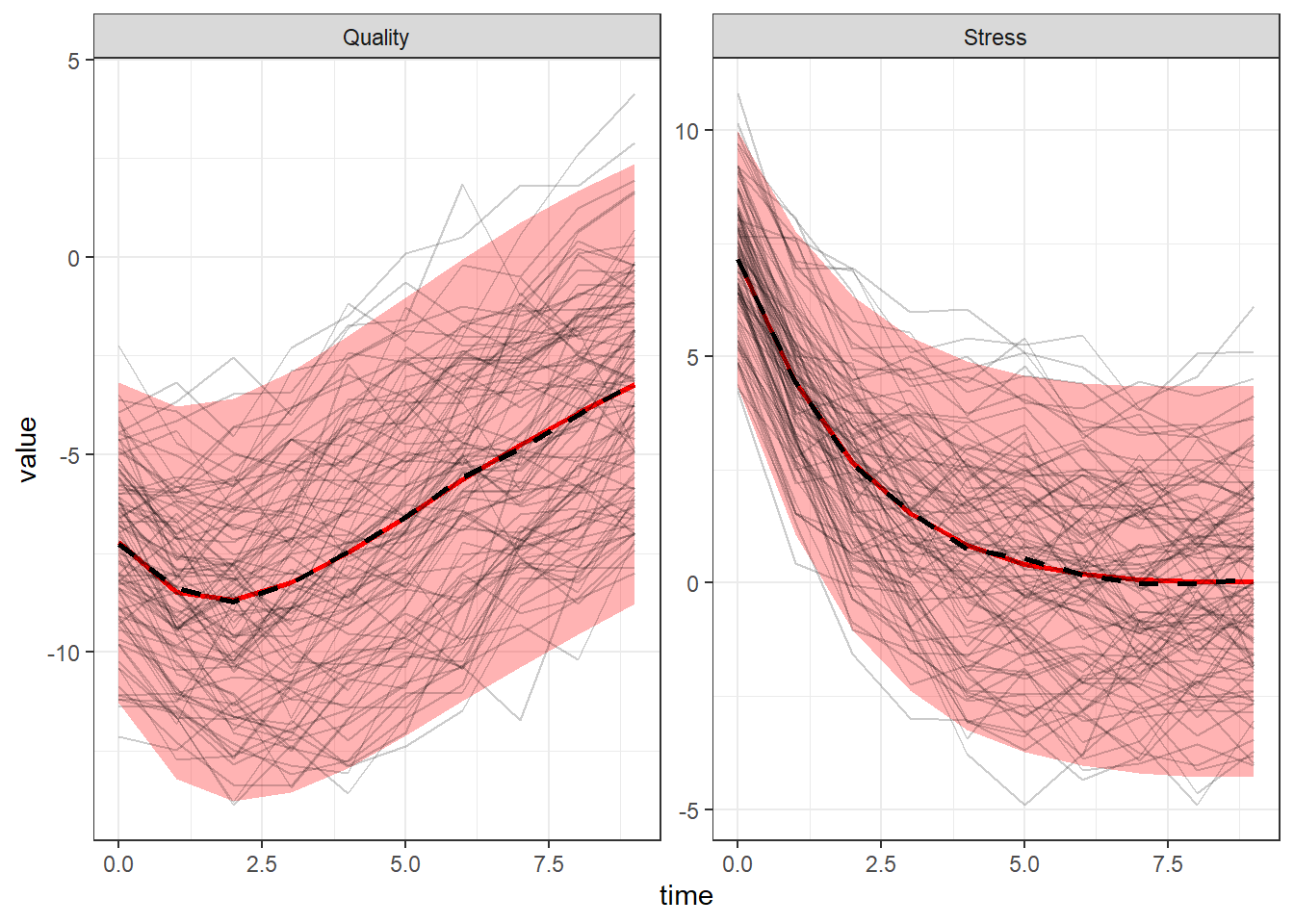

Residual Checks

We can extract the residuals and or standardised residuals from the model fit using the ctKalman function, then check for autocorrelation in the residuals – correlated residuals imply there is information left that our model did not leverage, meaning that our model could be improved. Here we show the autocorrelation using a method that treats time continuously, as well as the standard discrete-time approach in R. Here again our model is doing fine, the residual autocorrelation is approximately zero, there is no information remaining from the earlier time points to predict the latter.

k=ctKalman(fit,subjects=unique(dat$id)) #get residuals and various estimates
k=k[k$Element %in% 'errstdprior',] #remove everything except the residuals
k=dcast(data = data.table(k),formula = formula('Subject + Time ~ Row')) #cast to wider format

#continuous time auto and cross correlation
library(expct) #devtools::install_github("ryanoisin/expct") 
expct(dataset = k,Time = 'Time',ID = 'Subject',outcome=c('Quality'),
  plot_show = T,Tpred = 1:10,k = 5) #autocorrelation of residuals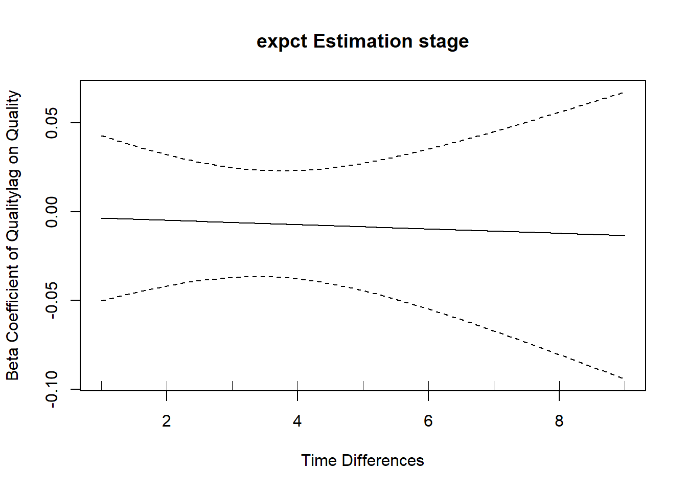 

#discrete time auto correlation
acf(k$Quality,lag.max=10,plot=TRUE)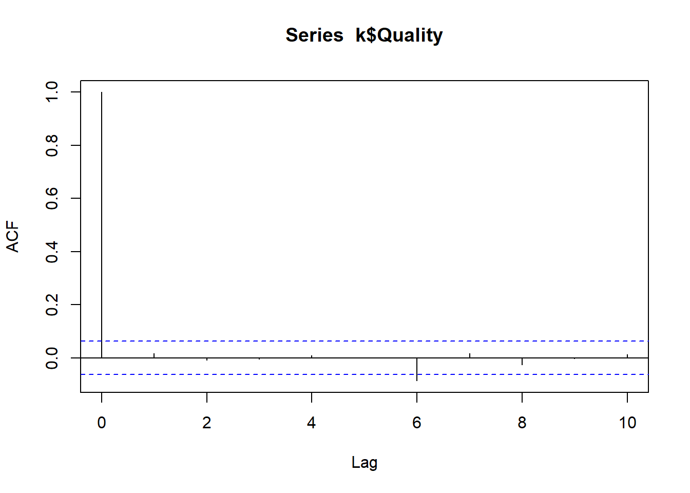

Factor / Measurement Models

Extending to a factor model formulation, using the additional measurement of stress we obtained, looks as follows, this time relying heavily on ctsem defaults for the free parameter specifications:

factormodel <- ctModel(type = 'standt',
  manifestNames = c('Stress','Stress2','Quality'), 
  LAMBDA = matrix(c(  #factor loadings / measurement structure 
    1,0,
    'stressLoading',0, #now with estimated factor loading for Stress2 variable
    0,1),ncol=2))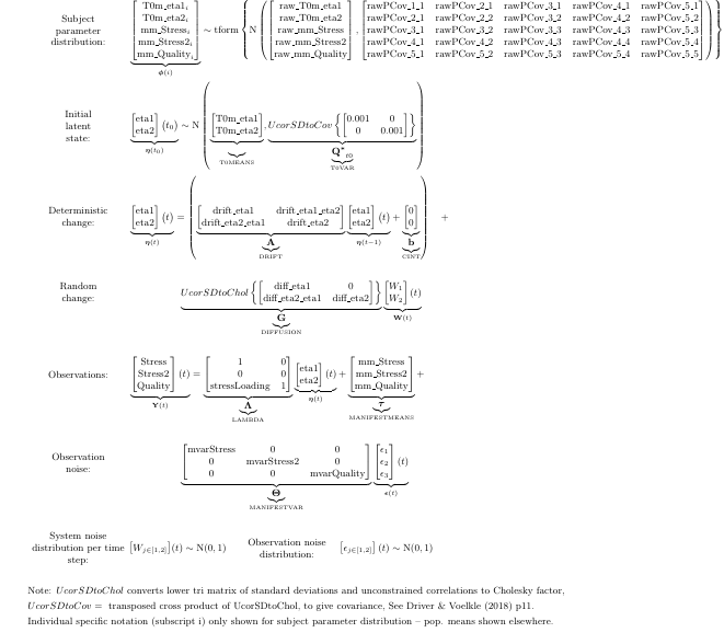

If we wanted to allow for stable individual variation only in the latent processes, and not in the measurement intercept, we would need to free the latent, or continuous, intercept (CINT, because it is added at each step), restrict all but one of the manifest intercepts (MANIFESTMEANS) to zero, and remove the individual variation from the estimated manifest intercept. Like this:

factormodellatent <- ctModel(type = 'standt',   
  manifestNames = c('Stress','Stress2','Quality'),
  LAMBDA = matrix(c(  #factor loadings / measurement structure 
    1,0,
    'stressLoading',0, #now with estimated factor loading for Stress2 variable
    0,1), ncol=2),
  CINT=c('cintStress','cintQuality'),
  MANIFESTMEANS=c(0,'mintStress2||FALSE',0)) #note the two || and FALSE, disabling individual variation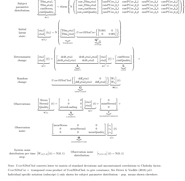

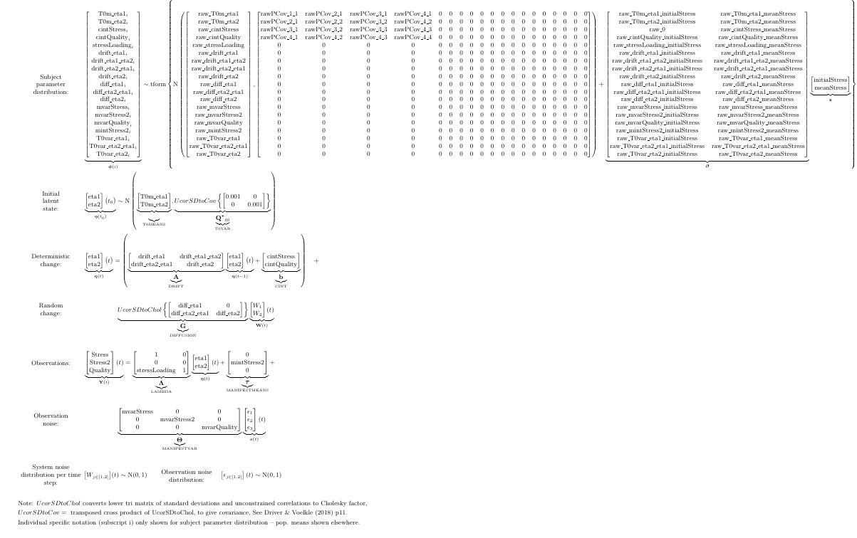
Want to account for heterogeneity in the model parameters without going wild and adding random effects (via the ||TRUE notation) to everything? Including the initial values and or mean of the observations as moderators of the parameters is one possibility. Here we first compute initial and mean values for our dataset, then include them as time independent predictors (covariate moderators). We also allow for random effects in the free factor loading – maybe not totally sensible in this case but simply as a demonstration how to add random effects to other parameters.

require(data.table)
dat <- data.table(dat)
dat[,initialStress:=mean(c(Stress[1],Stress2[1])),by=id]
dat[,meanStress:=mean(c(Stress,Stress2)),by=id]
head(dat)

factormodellatentmod<- ctModel(type = 'standt', 
  TIpredNames = c('initialStress','meanStress'), 
  tipredDefault = TRUE, #by default, moderate all parameters
  CINT=c('cintStress||||meanStress', #only moderate cintStress using meanStress
    'cintQuality||||initialStress, meanStress'), #explicitly moderate via both covariates
  manifestNames = c('Stress','Stress2','Quality'),
  LAMBDA = matrix(c(  #factor loadings / measurement structure 
    1,0,
    'stressLoading||TRUE',0, #estimated factor loading for Stress2 variable, now as random effect
    0,1), ncol=2),
  MANIFESTMEANS=c(0,'mintStress2||FALSE',0)) #note the two || and FALSE, disabling individual variation

The matrices for individual differences get pretty big now, zoom in if you like…